Control Package Examples

Given below, are some comprehensive textbook examples to demonstrate the possible use cases of the Control Module.

Example 1

../../_images/Control_Problems_Q1.svg

A pole zero plot of an unknown Transfer Function is given above.

  1. Determine the exact Transfer Function if the continuous time DC Gain of the system is 20.

  2. Is the TransferFunction stable or unstable in nature.

  3. Obtain the unit impulse response of the system.

  4. Find the initial value of the time-domain response of system without using the time domain equation.

Solution

>>> # Imports
>>> from sympy import symbols, I, limit, pprint, solve, oo
>>> from sympy.physics.control import TransferFunction

Subpart 1

>>> s, k = symbols('s k')
>>> gain = k                        # Let unknwon gain be k
>>> a = [-3]                        # Zero at -3 in S plane
>>> b = [-1, -2-I, -2+I]            # Poles at -1, (-2, j) and (-2, -j) in S plane
>>> tf = TransferFunction.from_zpk(a, b, gain, s)
>>> pprint(tf)
           k*(s + 3)
-------------------------------
(s + 1)*(s + 2 - I)*(s + 2 + I)
>>> gain = tf.dc_gain()
>>> print(gain)
3*k*(2 - I)*(2 + I)/25
>>> K = solve(gain - 20, k)[0]               # Solve for k
>>> tf = tf.subs({k: K})                     # Reconstruct the TransferFunction using .subs()
>>> pprint(tf.expand())
   100*s
   ----- + 100
     3
-------------------
 3      2
s  + 5*s  + 9*s + 5

Subpart 2

>>> tf.is_stable()  # Expect True, since poles lie in the left half of S plane
True

Subpart 3

>>> from sympy import inverse_laplace_transform
>>> t = symbols('t', positive = True)
>>> # Convert from S to T domain for impulse response
>>> tf = tf.to_expr()
>>> Impulse_Response = inverse_laplace_transform(tf, s, t)
>>> pprint(Impulse_Response)
      -t        -2*t
 100*e     100*e    *cos(t)
 ------- - ----------------
    3             3

Subpart 4

>>> # Apply the Initial Value Theorem on Equation of S domain
>>> # limit(y(t), t, 0) = limit(s*Y(S), s, oo)
>>> limit(s*tf, s, oo)
0

Example 2

Find the Transfer Function of the following Spring-Mass dampering system :

../../_images/Control_Problems_Q2.svg

Solution

>>> # Imports
>>> from sympy import Function, laplace_transform, laplace_initial_conds, laplace_correspondence, diff, Symbol, solve
>>> from sympy.abc import s, t
>>> from sympy.physics.control import TransferFunction
>>> y = Function('y')
>>> Y = Function('Y')
>>> u = Function('u')
>>> U = Function('U')
>>> k = Symbol('k') # Spring Constant
>>> c = Symbol('c') # Damper
>>> m = Symbol('m') # Mass of block

The DIFFERENTIAL EQUATION of the system will be as follows:

\[\begin{split}\frac{{d^2y(t)}}{{dt^2}} + c\frac{{dy(t)}}{{dt}} + ky(t) = w^2u(t) \\\\ with \ initial \ conditions \\ y(0) = t,\quad\frac{{dy}}{{dt}}\bigg|_{t=0} = 0\\\end{split}\]
>>> f = m*diff(y(t), t, t) + c*diff(y(t), t) + k*y(t) - u(t)
>>> F = laplace_transform(f, t, s, noconds=True)
>>> F = laplace_correspondence(F, {u: U, y: Y})
>>> F = laplace_initial_conds(F, t, {y: [0, 0]})
>>> t = (solve(F, Y(s))[0])/U(s) # To construct Transfer Function from Y(s) and U(s)
>>> tf = TransferFunction.from_rational_expression(t, s)
>>> pprint(tf)
      1
--------------
             2
c*s + k + m*s

Example 3

A signal matrix in the time-domain, also known as the impulse response matrix g(t) is given below.

\[\begin{split}g(t) = \begin{bmatrix} (1-t)e^{-t} & e^{-2t} \\ -e^{-t}+5e^{-2t} & \left(-3\sqrt{3}\sin\left(\frac{\sqrt{3}t}{2}\right)+\cos\left(\frac{\sqrt{3}t}{2}\right)\right)e^{-\frac{t}{2}} \end{bmatrix}\end{split}\]

With Respect to this matrix, find

  1. The system matrix (Transfer Function Matrix) in the Laplace domain (g(t)G(s)).

  2. The number of input and output signals in the system.

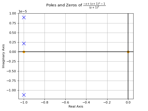
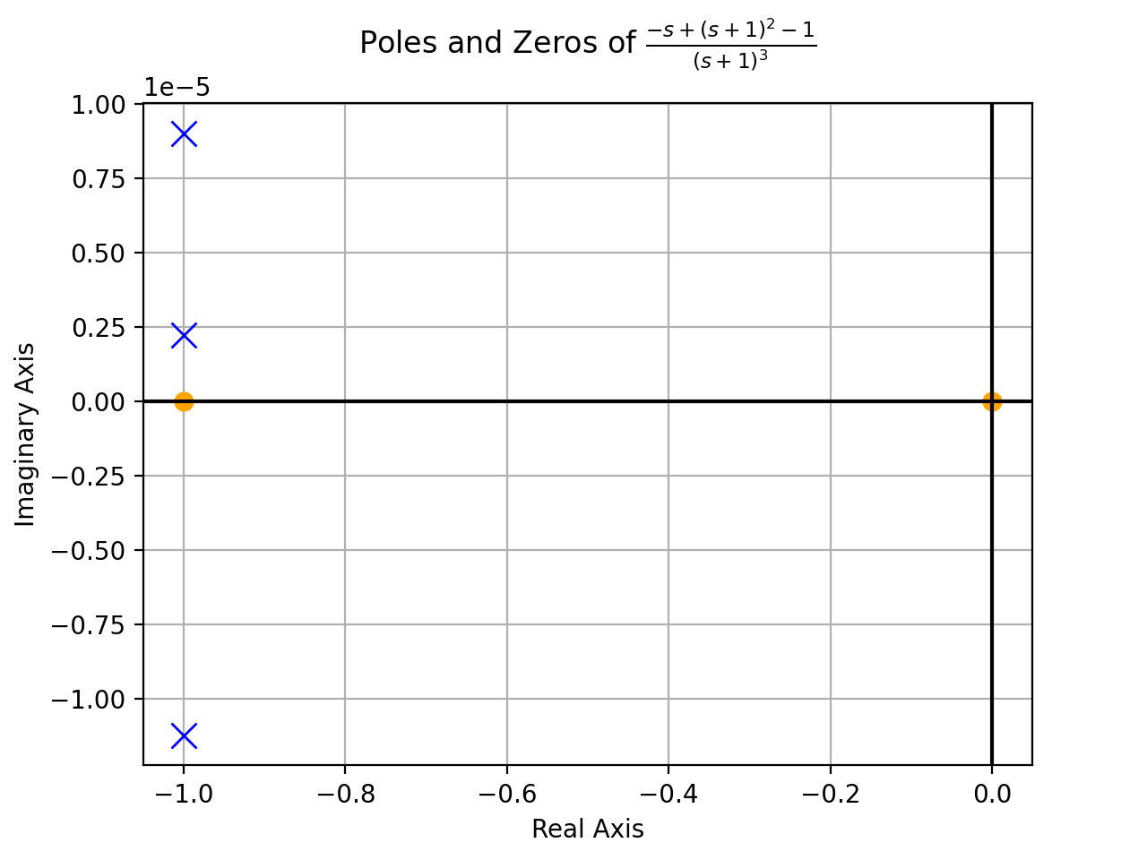
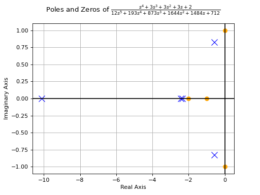
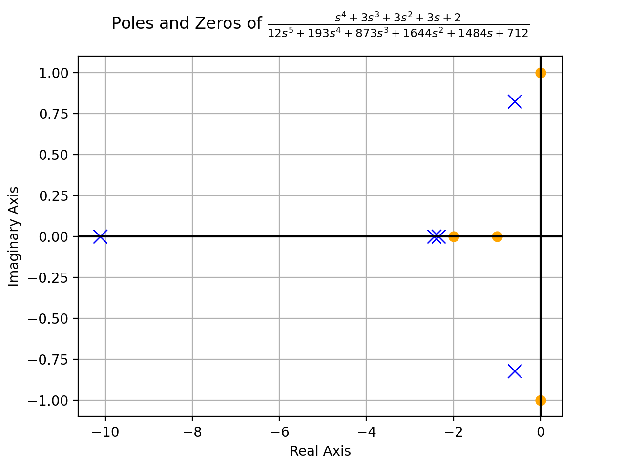
  3. Poles and Zeros of the system elements (individual Transfer Functions in Transfer Function Matrix) in the Laplace domain (Note: The actual poles and zeros of a MIMO system are NOT the poles and zeros of the individual elements of the transfer function matrix). Also, visualise the poles and zeros of the individual transfer function corresponding to the 1st input and 1st output of the G(s) matrix.

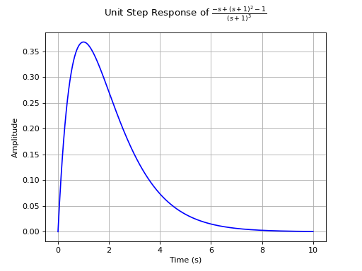
  4. Plot the unit step response of the individual Transfer Function corresponding to the 1st input and 1st output of the G(s) matrix.

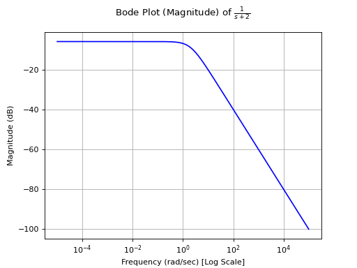
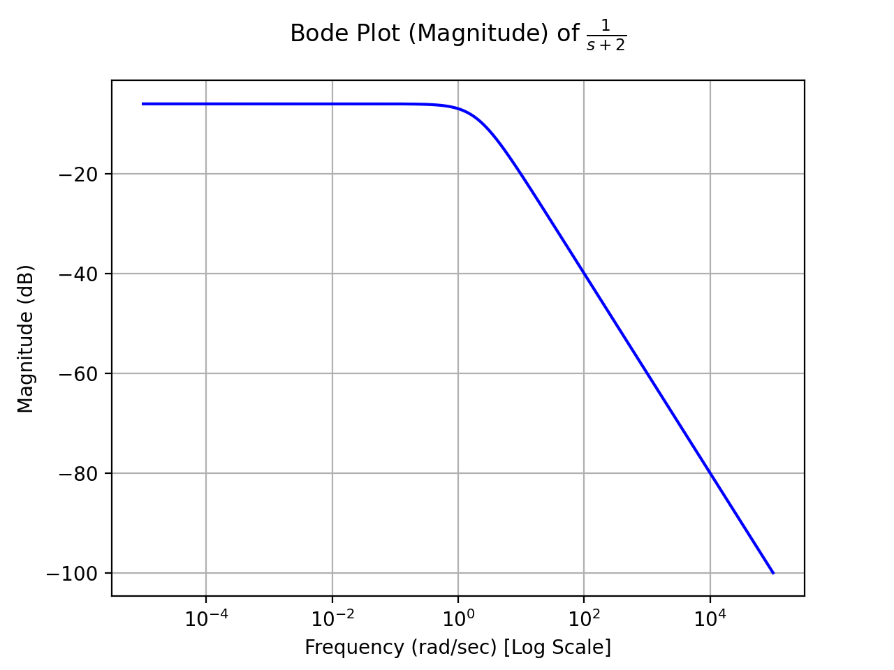
  5. Analyse the Bode magnitude and phase plot of the Transfer Function corresponding to 1st input and 2nd output of the G(s) matrix.

Solution

>>> # Imports
>>> from sympy import Matrix, laplace_transform, inverse_laplace_transform, exp, cos, sqrt, sin, pprint
>>> from sympy.abc import s, t
>>> from sympy.physics.control import *

Subpart 1

>>> g =  Matrix([[exp(-t)*(1 - t), exp(-2*t)], [5*exp((-2*t))-exp((-t)), (cos((sqrt(3)*t)/2) - 3*sqrt(3)*sin((sqrt(3)*t)/2))*exp(-t/2)]])
>>> G = g.applyfunc(lambda a: laplace_transform(a, t, s)[0])
>>> pprint(G)
[  1        1                       1                 ]
[----- - --------                 -----               ]
[s + 1          2                 s + 2               ]
[        (s + 1)                                      ]
[                                                     ]
[   5       1         s + 1/2               9         ]
[ ----- - -----    -------------- - ------------------]
[ s + 2   s + 1             2   3     /         2   3\]
[                  (s + 1/2)  + -   2*|(s + 1/2)  + -|]
[                               4     \             4/]

Subpart 2

>>> G = TransferFunctionMatrix.from_Matrix(G, s)
>>> type(G)
<class 'sympy.physics.control.lti.TransferFunctionMatrix'>
>>> type(G[0])
<class 'sympy.physics.control.lti.TransferFunction'>
>>> print(f'Inputs = {G.num_inputs}, Outputs = {G.num_outputs}')
Inputs = 2, Outputs = 2

Subpart 3

>>> G.elem_poles()
[[[-1, -1, -1], [-2]], [[-2, -1], [-1/2 - sqrt(3)*I/2, -1/2 - sqrt(3)*I/2, -1/2 + sqrt(3)*I/2, -1/2 + sqrt(3)*I/2]]]
>>> G.elem_zeros()
[[[-1, 0], []], [[-3/4], [4, -1/2 - sqrt(3)*I/2, -1/2 + sqrt(3)*I/2]]]
>>> pole_zero_plot(G[0, 0])   

(png, hires.png, pdf)

../../_images/generate_plots_q3_3.png

Subpart 4

>>> tf1 = G[0, 0]
>>> pprint(tf1)
            2
-s + (s + 1)  - 1
-----------------
            3
     (s + 1)
>>> step_response_plot(tf1)  

(png, hires.png, pdf)

../../_images/generate_plots_q3_4.png

Subpart 5

>>> tf2 = G[0, 1]
>>> bode_magnitude_plot(tf2)  

(png, hires.png, pdf)

../../_images/generate_plots_q3_5_1.png
>>> bode_phase_plot(tf2)  

(png, hires.png, pdf)

../../_images/generate_plots_q3_5_2.png

Example 4

  1. A system is designed by arranging P(s) and C(s) in a series configuration (Values of P(s) and C(s) are provided below). Compute the equivalent system matrix, when the order of blocks is reversed (i.e. C(s) then P(s)).

    \[\begin{split}P(s) = \begin{bmatrix} \frac{1}{s} & \frac{2}{s+2} \\ 0 & 3 \end{bmatrix}\end{split}\]

    \[\begin{split}C(s) = \begin{bmatrix} 1 & 1 \\ 2 & 2 \end{bmatrix}\end{split}\]

  2. Also, find the equivalent closed-loop system (or the ratio v/u from the block diagram given below) for the system (negative-feedback loop) having C(s) as the controller and P(s) as plant (Refer to the block diagram given below).

    ../../_images/Control_Problems_Q4.svg

Solution

>>> # Imports
>>> from sympy import Matrix, pprint
>>> from sympy.abc import s, t
>>> from sympy.physics.control import *

Subpart 1

>>> P_mat = Matrix([[1/s, 2/(2+s)], [0, 3]])
>>> C_mat = Matrix([[1, 1], [2, 2]])
>>> P = TransferFunctionMatrix.from_Matrix(P_mat, var=s)
>>> C = TransferFunctionMatrix.from_Matrix(C_mat, var=s)
>>> # Series equivalent, considering (Input)→[P]→[C]→(Output). Note that order of matrix multiplication is opposite to the order in which the elements are arranged.
>>> pprint(C*P)
[1  1]    [1    2  ]
[-  -]    [-  -----]
[1  1]    [s  s + 2]
[    ]   *[        ]
[2  2]    [0    3  ]
[-  -]    [-    -  ]
[1  1]{t} [1    1  ]{t}
>>> # Series equivalent, considering (Input)→[C]→[P]→(Output).
>>> pprint(P*C)
[1    2  ]    [1  1]
[-  -----]    [-  -]
[s  s + 2]    [1  1]
[        ]   *[    ]
[0    3  ]    [2  2]
[-    -  ]    [-  -]
[1    1  ]{t} [1  1]{t}
>>> pprint((C*P).doit())
[1  3*s + 8 ]
[-  ------- ]
[s   s + 2  ]
[           ]
[2  6*s + 16]
[-  --------]
[s   s + 2  ]{t}
>>> pprint((P*C).doit())
[ 5*s + 2    5*s + 2 ]
[---------  ---------]
[s*(s + 2)  s*(s + 2)]
[                    ]
[    6          6    ]
[    -          -    ]
[    1          1    ]{t}

Subpart 2

>>> tfm_feedback = MIMOFeedback(P, C, sign=-1)
>>> pprint(tfm_feedback.doit())  # ((I + P*C)**-1)*P
[   7*s + 14          -s - 6     ]
[---------------  ---------------]
[   2                2           ]
[7*s  + 19*s + 2  7*s  + 19*s + 2]
[                                ]
[                    2           ]
[   -6*s - 12     3*s  + 9*s + 6 ]
[---------------  ---------------]
[   2                2           ]
[7*s  + 19*s + 2  7*s  + 19*s + 2]{t}

Example 5

../../_images/Control_Problems_Q5.svg

Given,

\[ \begin{align}\begin{aligned}\begin{split}G1 &= \frac{1}{10 + s}\\\\\end{split}\\\begin{split}G2 &= \frac{1}{1 + s}\\\\\end{split}\\\begin{split}G3 &= \frac{1 + s^2}{4 + 4s + s^2}\\\\\end{split}\\\begin{split}G4 &= \frac{1 + s}{6 + s}\\\\\end{split}\\\begin{split}H1 &= \frac{1 + s}{2 + s}\\\\\end{split}\\\begin{split}H2 &= \frac{2 \cdot (6 + s)}{1 + s}\\\\\end{split}\\\begin{split}H3 &= 1\\\end{split}\end{aligned}\end{align} \]

Where \(s\) is the variable of the transfer function (in Laplace Domain).

Find

  1. The equivalent Transfer Function representing the system given above.

  2. Pole-Zero plot of the system.

Solution

>>> from sympy.abc import s
>>> from sympy.physics.control import *
>>> G1 = TransferFunction(1, 10 + s, s)
>>> G2 = TransferFunction(1, 1 + s, s)
>>> G3 = TransferFunction(1 + s**2, 4 + 4*s + s**2, s)
>>> G4 = TransferFunction(1 + s, 6 + s, s)
>>> H1 = TransferFunction(1 + s, 2 + s, s)
>>> H2 = TransferFunction(2*(6 + s), 1 + s, s)
>>> H3 = TransferFunction(1, 1, s)
>>> sys1 = Series(G3, G4)
>>> sys2 = Feedback(sys1, H1, 1).doit()
>>> sys3 = Series(G2, sys2)
>>> sys4 = Feedback(sys3, H2).doit()
>>> sys5 = Series(G1, sys4)
>>> sys6 = Feedback(sys5, H3)
>>> sys6  # Final unevaluated Feedback object
Feedback(Series(TransferFunction(1, s + 10, s), TransferFunction((s + 1)**3*(s + 2)*(s + 6)**2*(s**2 + 1)*(-(s + 1)**2*(s**2 + 1) + (s + 2)*(s + 6)*(s**2 + 4*s + 4))*(s**2 + 4*s + 4)**2, (s + 1)*(s + 6)*(-(s + 1)**2*(s**2 + 1) + (s + 2)*(s + 6)*(s**2 + 4*s + 4))*((s + 1)**2*(s + 6)*(-(s + 1)**2*(s**2 + 1) + (s + 2)*(s + 6)*(s**2 + 4*s + 4))*(s**2 + 4*s + 4) + (s + 1)*(s + 2)*(s + 6)*(2*s + 12)*(s**2 + 1)*(s**2 + 4*s + 4))*(s**2 + 4*s + 4), s)), TransferFunction(1, 1, s), -1)
>>> sys6.doit()  # Reducing to TransferFunction form without simplification
TransferFunction((s + 1)**4*(s + 2)*(s + 6)**3*(s + 10)*(s**2 + 1)*(-(s + 1)**2*(s**2 + 1) + (s + 2)*(s + 6)*(s**2 + 4*s + 4))**2*((s + 1)**2*(s + 6)*(-(s + 1)**2*(s**2 + 1) + (s + 2)*(s + 6)*(s**2 + 4*s + 4))*(s**2 + 4*s + 4) + (s + 1)*(s + 2)*(s + 6)*(2*s + 12)*(s**2 + 1)*(s**2 + 4*s + 4))*(s**2 + 4*s + 4)**3, (s + 1)*(s + 6)*(s + 10)*(-(s + 1)**2*(s**2 + 1) + (s + 2)*(s + 6)*(s**2 + 4*s + 4))*((s + 1)**2*(s + 6)*(-(s + 1)**2*(s**2 + 1) + (s + 2)*(s + 6)*(s**2 + 4*s + 4))*(s**2 + 4*s + 4) + (s + 1)*(s + 2)*(s + 6)*(2*s + 12)*(s**2 + 1)*(s**2 + 4*s + 4))*((s + 1)**3*(s + 2)*(s + 6)**2*(s**2 + 1)*(-(s + 1)**2*(s**2 + 1) + (s + 2)*(s + 6)*(s**2 + 4*s + 4))*(s**2 + 4*s + 4)**2 + (s + 1)*(s + 6)*(s + 10)*(-(s + 1)**2*(s**2 + 1) + (s + 2)*(s + 6)*(s**2 + 4*s + 4))*((s + 1)**2*(s + 6)*(-(s + 1)**2*(s**2 + 1) + (s + 2)*(s + 6)*(s**2 + 4*s + 4))*(s**2 + 4*s + 4) + (s + 1)*(s + 2)*(s + 6)*(2*s + 12)*(s**2 + 1)*(s**2 + 4*s + 4))*(s**2 + 4*s + 4))*(s**2 + 4*s + 4), s)
>>> sys6 = sys6.doit(cancel=True, expand=True)  # Simplified TransferFunction form
>>> sys6
TransferFunction(s**4 + 3*s**3 + 3*s**2 + 3*s + 2, 12*s**5 + 193*s**4 + 873*s**3 + 1644*s**2 + 1484*s + 712, s)
>>> pole_zero_plot(sys6)  

(png, hires.png, pdf)

../../_images/generate_plots_q5.png

References

  1. testbook.com

  2. www.vssut.ac.in