Solve an Ordinary Differential Equation (ODE) Algebraically
Use SymPy to solve an ordinary differential equation (ODE) algebraically. For example, solving \(y''(x) + 9y(x)=0 \) yields \( y(x)=C_{1} \sin(3x)+ C_{2} \cos(3x)\).
Alternatives to Consider
To numerically solve a system of ODEs, use a SciPy ODE solver such as
solve_ivp. You can also use SymPy to create and thenlambdify()an ODE to be solved numerically using SciPy’s assolve_ivpas described below in Numerically Solve an ODE in SciPy.
Solve an Ordinary Differential Equation (ODE)
Here is an example of solving the above ordinary differential equation
algebraically using dsolve(). You can then use checkodesol() to
verify that the solution is correct.
>>> from sympy import Function, dsolve, Derivative, checkodesol
>>> from sympy.abc import x
>>> y = Function('y')
>>> # Solve the ODE
>>> result = dsolve(Derivative(y(x), x, x) + 9*y(x), y(x))
>>> result
Eq(y(x), C1*sin(3*x) + C2*cos(3*x))
>>> # Check that the solution is correct
>>> checkodesol(Derivative(y(x), x, x) + 9*y(x), result)
(True, 0)
The output of checkodesol() is a tuple where the first item, a boolean,
tells whether substituting the solution into the ODE results in 0, indicating
the solution is correct.
Guidance
Defining Derivatives
There are many ways to express derivatives of functions. For an undefined
function, both Derivative and diff() represent the undefined
derivative. Thus, all of the following ypp (“y prime prime”) represent \(y''\),
the second derivative with respect to \(x\) of a function \(y(x)\):
ypp = y(x).diff(x, x)
ypp = y(x).diff(x, 2)
ypp = y(x).diff((x, 2))
ypp = diff(y(x), x, x)
ypp = diff(y(x), x, 2)
ypp = Derivative(y(x), x, x)
ypp = Derivative(y(x), x, 2)
ypp = Derivative(Derivative(y(x), x), x)
ypp = diff(diff(y(x), x), x)
yp = y(x).diff(x)
ypp = yp.diff(x)
We recommend specifying the function to be solved for, as the second argument to
dsolve(). Note that it must be a function rather than a variable
(symbol). SymPy will give an error if you specify a variable (\(x\)) rather than a
function (\(f(x)\)):
>>> dsolve(Derivative(y(x), x, x) + 9*y(x), x)
Traceback (most recent call last):
    ...
ValueError: dsolve() and classify_ode() only work with functions of one variable, not x
Similarly, you must specify the argument of the function: \(y(x)\), not just \(y\).
Options to Define an ODE
You can define the function to be solved for in two ways. The subsequent syntax for specifying initial conditions depends on your choice.
Option 1: Define a Function Without Including Its Independent Variable
You can define a function without including its independent variable:
>>> from sympy import symbols, Eq, Function, dsolve
>>> f, g = symbols("f g", cls=Function)
>>> x = symbols("x")
>>> eqs = [Eq(f(x).diff(x), g(x)), Eq(g(x).diff(x), f(x))]
>>> dsolve(eqs, [f(x), g(x)])
[Eq(f(x), -C1*exp(-x) + C2*exp(x)), Eq(g(x), C1*exp(-x) + C2*exp(x))]
Note that you supply the functions to be solved for as a list as the second
argument of dsolve(), here [f(x), g(x)].
Specify Initial Conditions or Boundary Conditions
If your differential equation(s) have initial or boundary conditions, specify
them with the dsolve() optional argument ics. Initial and boundary
conditions are treated the same way (even though the argument is called ics).
It should be given in the form of {f(x0): y0, f(x).diff(x).subs(x, x1): y1}
and so on where, for example, the value of \(f(x)\) at \(x = x_{0}\) is \(y_{0}\). For
power series solutions, if no initial conditions are specified \(f(0)\) is assumed
to be \(C_{0}\) and the power series solution is calculated about \(0\).
Here is an example of setting the initial values for functions, namely namely \(f(0) = 1\) and \(g(2) = 3\):
>>> from sympy import symbols, Eq, Function, dsolve
>>> f, g = symbols("f g", cls=Function)
>>> x = symbols("x")
>>> eqs = [Eq(f(x).diff(x), g(x)), Eq(g(x).diff(x), f(x))]
>>> dsolve(eqs, [f(x), g(x)])
[Eq(f(x), -C1*exp(-x) + C2*exp(x)), Eq(g(x), C1*exp(-x) + C2*exp(x))]
>>> dsolve(eqs, [f(x), g(x)], ics={f(0): 1, g(2): 3})
[Eq(f(x), (1 + 3*exp(2))*exp(x)/(1 + exp(4)) - (-exp(4) + 3*exp(2))*exp(-x)/(1 + exp(4))), Eq(g(x), (1 + 3*exp(2))*exp(x)/(1 + exp(4)) + (-exp(4) + 3*exp(2))*exp(-x)/(1 + exp(4)))]
Here is an example of setting the initial value for the derivative of a function, namely \(f'(1) = 2\):
>>> eqn = Eq(f(x).diff(x), f(x))
>>> dsolve(eqn, f(x), ics={f(x).diff(x).subs(x, 1): 2})
Eq(f(x), 2*exp(-1)*exp(x))
Option 2: Define a Function of an Independent Variable
You may prefer to specify a function (for example \(y\)) of its independent
variable (for example \(t\)), so that y represents y(t):
>>> from sympy import symbols, Function, dsolve
>>> t = symbols('t')
>>> y = Function('y')(t)
>>> y
y(t)
>>> yp = y.diff(t)
>>> ypp = yp.diff(t)
>>> eq = ypp + 2*yp + y
>>> eq
y(t) + 2*Derivative(y(t), t) + Derivative(y(t), (t, 2))
>>> dsolve(eq, y)
Eq(y(t), (C1 + C2*t)*exp(-t))
Using this convention, the second argument of dsolve(), y, represents
y(t), so SymPy recognizes it as a valid function to solve for.
Specify Initial Conditions or Boundary Conditions
Using that syntax, you specify initialor boundary conditions by substituting in
values of the independent variable using subs()
because the function \(y\) already has its independent variable as an argument
\(t\):
>>> dsolve(eq, y, ics={y.subs(t, 0): 0})
Eq(y(t), C2*t*exp(-t))
Beware Copying and Pasting Results
If you choose to define a function of an independent variable, note that copying
a result and pasting it into subsequent code may cause an error because x is
already defined as y(t), so if you paste in y(t) it is interpreted as
y(t)(t):
>>> dsolve(y(t).diff(y), y)
Traceback (most recent call last):
    ...
TypeError: 'y' object is not callable
So remember to exclude the independent variable call (t):
>>> dsolve(y.diff(t), y)
Eq(y(t), C1)
Use the Solution Result
Unlike other solving functions, dsolve() returns an Equality
(equation) formatted as, for example, Eq(y(x), C1*sin(3*x) + C2*cos(3*x))
which is equivalent to the mathematical notation \(y(x) = C_1 \sin(3x) + C_2
\cos(3x)\).
Extract the Result for One Solution and Function
You can extract the result from an Equality using the right-hand side
property rhs:
>>> from sympy import Function, dsolve, Derivative
>>> from sympy.abc import x
>>> y = Function('y')
>>> result = dsolve(Derivative(y(x), x, x) + 9*y(x), y(x))
>>> result
Eq(y(x), C1*sin(3*x) + C2*cos(3*x))
>>> result.rhs
C1*sin(3*x) + C2*cos(3*x)
Some ODEs Cannot Be Solved Explicitly, Only Implicitly
The above ODE can be solved explicitly, specifically \(y(x)\) can be expressed in terms of functions of \(x\). However, some ODEs cannot be solved explicitly, for example:
>>> from sympy import dsolve, exp, symbols, Function
>>> f = symbols("f", cls=Function)
>>> x = symbols("x")
>>> dsolve(f(x).diff(x) + exp(-f(x))*f(x))
Eq(Ei(f(x)), C1 - x)
This gives no direct expression for \(f(x)\). Instead, dsolve() expresses
a solution as \(g(f(x))\) where \(g\) is Ei, the classical exponential
integral function. Ei does not have a known closed-form inverse, so a solution
cannot be explicitly expressed as \(f(x)\) equaling a function of \(x\). Instead,
dsolve returns an implicit
solution.
When dsolve returns an implicit solution, extracting the right-hand side of
the returned equality will not give an explicitly expression for the function to
be solved for, here \(f(x)\). So before extracting an expression for the function
to be solved for, check that dsolve was able to solve for the function
explicitly.
Extract the Result for Multiple Function-Solution Pairs
If you are solving a system of equations with multiple unknown functions, the
form of the output of dsolve() depends on whether there is one or
multiple solutions.
If There is One Solution Set
If there is only one solution set to a system of equations with multiple unknown
functions, dsolve() will return a non-nested list containing an
equality. You can extract the solution expression using a single loop or
comprehension:
>>> from sympy import symbols, Eq, Function, dsolve
>>> y, z = symbols("y z", cls=Function)
>>> x = symbols("x")
>>> eqs_one_soln_set = [Eq(y(x).diff(x), z(x)**2), Eq(z(x).diff(x), z(x))]
>>> solutions_one_soln_set = dsolve(eqs_one_soln_set, [y(x), z(x)])
>>> solutions_one_soln_set
[Eq(y(x), C1 + C2**2*exp(2*x)/2), Eq(z(x), C2*exp(x))]
>>> # Loop through list approach
>>> solution_one_soln_set_dict = {}
>>> for fn in solutions_one_soln_set:
...         solution_one_soln_set_dict.update({fn.lhs: fn.rhs})
>>> solution_one_soln_set_dict
{y(x): C1 + C2**2*exp(2*x)/2, z(x): C2*exp(x)}
>>> # List comprehension approach
>>> solution_one_soln_set_dict = {fn.lhs:fn.rhs for fn in solutions_one_soln_set}
>>> solution_one_soln_set_dict
{y(x): C1 + C2**2*exp(2*x)/2, z(x): C2*exp(x)}
>>> # Extract expression for y(x)
>>> solution_one_soln_set_dict[y(x)]
C1 + C2**2*exp(2*x)/2
If There are Multiple Solution Sets
If there are multiple solution sets to a system of equations with multiple
unknown functions, dsolve() will return a nested list of equalities, the
outer list representing each solution and the inner list representing each
function. While you can extract results by specifying the index of each
function, we recommend an approach which is robust with respect to function
ordering. The following converts each solution into a dictionary so you can
easily extract the result for the desired function. It uses standard Python
techniques such as loops or comprehensions, in a nested fashion.
>>> from sympy import symbols, Eq, Function, dsolve
>>> y, z = symbols("y z", cls=Function)
>>> x = symbols("x")
>>> eqs = [Eq(y(x).diff(x)**2, z(x)**2), Eq(z(x).diff(x), z(x))]
>>> solutions = dsolve(eqs, [y(x), z(x)])
>>> solutions
[[Eq(y(x), C1 - C2*exp(x)), Eq(z(x), C2*exp(x))], [Eq(y(x), C1 + C2*exp(x)), Eq(z(x), C2*exp(x))]]
>>> # Nested list approach
>>> solutions_list = []
>>> for solution in solutions:
...     solution_dict = {}
...     for fn in solution:
...             solution_dict.update({fn.lhs: fn.rhs})
...     solutions_list.append(solution_dict)
>>> solutions_list
[{y(x): C1 - C2*exp(x), z(x): C2*exp(x)}, {y(x): C1 + C2*exp(x), z(x): C2*exp(x)}]
>>> # Nested comprehension approach
>>> solutions_list = [{fn.lhs:fn.rhs for fn in solution} for solution in solutions]
>>> solutions_list
[{y(x): C1 - C2*exp(x), z(x): C2*exp(x)}, {y(x): C1 + C2*exp(x), z(x): C2*exp(x)}]
>>> # Extract expression for y(x)
>>> solutions_list[0][y(x)]
C1 - C2*exp(x)
Work With Arbitrary Constants
You can manipulate arbitrary constants such as C1, C2, and C3, which are
generated automatically by dsolve(), by creating them as symbols. For
example, if you want to assign values to arbitrary constants, you can create
them as symbols and then substitute in their values using
subs():
>>> from sympy import Function, dsolve, Derivative, symbols, pi
>>> y = Function('y')
>>> x, C1, C2 = symbols("x, C1, C2")
>>> result = dsolve(Derivative(y(x), x, x) + 9*y(x), y(x)).rhs
>>> result
C1*sin(3*x) + C2*cos(3*x)
>>> result.subs({C1: 7, C2: pi})
7*sin(3*x) + pi*cos(3*x)
Numerically Solve an ODE in SciPy
A common workflow which leverages SciPy’s fast numerical ODE solving is
set up an ODE in SymPy
convert it to a numerical function using
lambdify()solve the initial value problem by numerically integrating the ODE using SciPy’s
solve_ivp.
Here is an example from the field of chemical kinetics where the nonlinear ordinary differential equations take this form:
and
>>> from sympy import symbols, lambdify
>>> import numpy as np
>>> import scipy.integrate
>>> import matplotlib.pyplot as plt
>>> # Create symbols y0, y1, and y2
>>> y = symbols('y:3')
>>> kf, kb = symbols('kf kb')
>>> rf = kf * y[0]**2 * y[1]
>>> rb = kb * y[2]**2
>>> # Derivative of the function y(t); values for the three chemical species
>>> # for input values y, kf, and kb
>>> ydot = [2*(rb - rf), rb - rf, 2*(rf - rb)]
>>> ydot
[2*kb*y2**2 - 2*kf*y0**2*y1, kb*y2**2 - kf*y0**2*y1, -2*kb*y2**2 + 2*kf*y0**2*y1]
>>> t = symbols('t') # not used in this case
>>> # Convert the SymPy symbolic expression for ydot into a form that
>>> # SciPy can evaluate numerically, f
>>> f = lambdify((t, y, kf, kb), ydot)
>>> k_vals = np.array([0.42, 0.17]) # arbitrary in this case
>>> y0 = [1, 1, 0] # initial condition (initial values)
>>> t_eval = np.linspace(0, 10, 50) # evaluate integral from t = 0-10 for 50 points
>>> # Call SciPy's ODE initial value problem solver solve_ivp by passing it
>>> #   the function f,
>>> #   the interval of integration,
>>> #   the initial state, and
>>> #   the arguments to pass to the function f
>>> solution = scipy.integrate.solve_ivp(f, (0, 10), y0, t_eval=t_eval, args=k_vals)
>>> # Extract the y (concentration) values from SciPy solution result
>>> y = solution.y
>>> # Plot the result graphically using matplotlib
>>> plt.plot(t_eval, y.T)
>>> # Add title, legend, and axis labels to the plot
>>> plt.title('Chemical Kinetics')
>>> plt.legend(['NO', 'Br$_2$', 'NOBr'], shadow=True)
>>> plt.xlabel('time')
>>> plt.ylabel('concentration')
>>> # Finally, display the annotated plot
>>> plt.show()
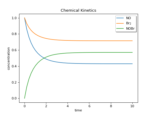
SciPy’s solve_ivp returns a result containing y (numerical function result,
here, concentration) values for each of the three chemical species,
corresponding to the time points t_eval.
Ordinary Differential Equation Solving Hints
Return Unevaluated Integrals
By default, dsolve() attempts to evaluate the integrals it produces to
solve your ordinary differential equation. You can disable evaluation of the
integrals by using Hint Functions ending with _Integral, for example
separable_Integral. This is useful because
integrate() is an expensive routine. SymPy may hang
(appear to never complete the operation) because of a difficult or impossible
integral, so using an _Integral hint will at least return an (unintegrated)
result, which you can then consider. The simplest way to disable integration is
with the all_Integral hint because you do not need to know which hint to
supply: for any hint with a corresponding _Integral hint, all_Integral only
returns the _Integral hint.
Select a Specific Solver
You may wish to select a specific solver using a hint for a couple of reasons:
educational purposes: for example if you are learning about a specific method to solve ODEs and want to get a result that exactly matches that method
form of the result: sometimes an ODE can be solved by many different solvers, and they can return different results. They will be mathematically equivalent, though the arbitrary constants may not be.
dsolve()by default tries to use the “best” solvers first, which are most likely to return the most usable output, but it is not a perfect heuristic. For example, the “best” solver may produce a result with an integral that SymPy cannot solve, but another solver may produce a different integral that SymPy can solve. So if the solution isn’t in a form you like, you can try other hints to check whether they give a preferable result.
Not All Equations Can Be Solved
Equations With No Solution
Not all differential equations can be solved, for example:
>>> from sympy import Function, dsolve, Derivative, symbols
>>> y = Function('y')
>>> x, C1, C2 = symbols("x, C1, C2")
>>> dsolve(Derivative(y(x), x, 3) - (y(x)**2), y(x)).rhs
Traceback (most recent call last):
    ...
NotImplementedError: solve: Cannot solve -y(x)**2 + Derivative(y(x), (x, 3))
Equations With No Closed-Form Solution
As noted above, Some ODEs Cannot Be Solved Explicitly, Only Implicitly.
Also, some systems of differential equations have no closed-form solution because they are chaotic, for example the Lorenz system or a double pendulum described by these two differential equations (simplified from ScienceWorld):
>>> from sympy import symbols, Function, cos, sin, dsolve
>>> theta1, theta2 = symbols('theta1 theta2', cls=Function)
>>> g, t = symbols('g t')
>>> eq1 = 2*theta1(t).diff(t, t) + theta2(t).diff(t, t)*cos(theta1(t) - theta2(t)) + theta2(t).diff(t)**2*sin(theta1(t) - theta2(t)) + 2*g*sin(theta1(t))
>>> eq2 = theta2(t).diff(t, t) + theta1(t).diff(t, t)*cos(theta1(t) - theta2(t)) - theta1(t).diff(t)**2*sin(theta1(t) - theta2(t)) + g*sin(theta2(t))
>>> dsolve([eq1, eq2], [theta1(t), theta2(t)])
Traceback (most recent call last):
...
NotImplementedError
For such cases, you can solve the equations numerically as mentioned in Alternatives to Consider.
Report a Bug
If you find a bug with dsolve(), please post the problem on the SymPy mailing
list. Until the issue is resolved, you can
use a different method listed in Alternatives to Consider.