Multi Degree of Freedom Holonomic System
In this example we demonstrate the use of the functionality provided in
sympy.physics.mechanics for deriving the equations of motion (EOM) of a
holonomic system that includes both particles and rigid bodies with contributing
forces and torques, some of which are specified forces and torques. The system
is shown below:
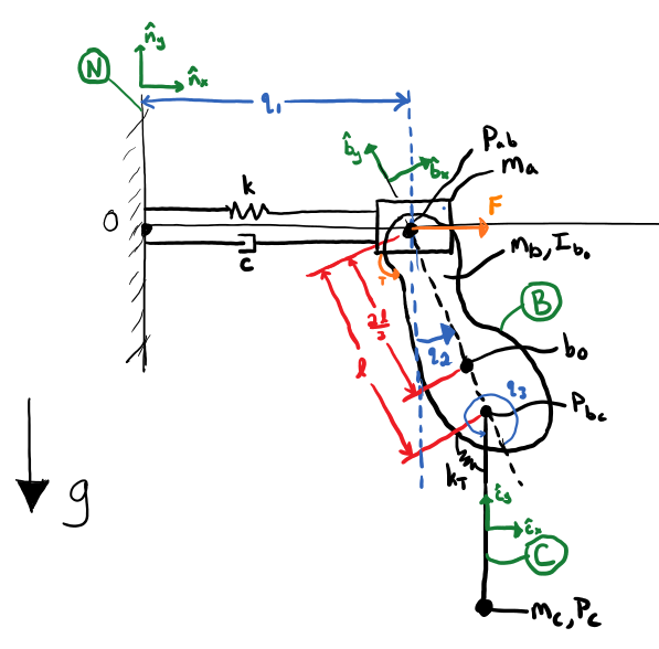
The system will be modeled using System. First we need to create the
dynamicsymbols() needed to describe the system as shown in the above
diagram. In this case, the generalized coordinates \(q_1\) represent lateral
distance of block from wall, \(q_2\) represents angle of the compound
pendulum from vertical, \(q_3\) represents angle of the simple pendulum
from the compound pendulum. The generalized speeds \(u_1\) represents
lateral speed of block, \(u_2\) represents lateral speed of compound
pendulum and \(u_3\) represents angular speed of C relative to B.
We also create some symbols() to represent the length and mass of the
pendulum, as well as gravity and others.
>>> from sympy import zeros, symbols
>>> from sympy.physics.mechanics import *
>>> q1, q2, q3, u1, u2, u3 = dynamicsymbols('q1, q2, q3, u1, u2, u3')
>>> F, T = dynamicsymbols('F, T')
>>> l, k, c, g, kT = symbols('l, k, c, g, kT')
>>> ma, mb, mc, IBzz= symbols('ma, mb, mc, IBzz')
With all symbols defined, we can now define the bodies and initialize our
instance of System.
>>> wall = RigidBody('N')
>>> block = Particle('A', mass=ma)
>>> compound_pend = RigidBody('B', mass=mb)
>>> compound_pend.central_inertia = inertia(compound_pend.frame, 0, 0, IBzz)
>>> simple_pend = Particle('C', mass=mc)
>>> system = System.from_newtonian(wall)
>>> system.add_bodies(block, compound_pend, simple_pend)
Next, we connect the bodies using joints to establish the kinematics. Note that we specify the intermediate frames for both particles, as particles do not have an associated frame.
>>> block_frame = ReferenceFrame('A')
>>> block.masscenter.set_vel(block_frame, 0)
>>> slider = PrismaticJoint('J1', wall, block, coordinates=q1, speeds=u1,
...                         child_interframe=block_frame)
>>> rev1 = PinJoint('J2', block, compound_pend, coordinates=q2, speeds=u2,
...                 joint_axis=wall.z, child_point=l*2/3*compound_pend.y,
...                 parent_interframe=block_frame)
>>> simple_pend_frame = ReferenceFrame('C')
>>> simple_pend.masscenter.set_vel(simple_pend_frame, 0)
>>> rev2 = PinJoint('J3', compound_pend, simple_pend, coordinates=q3,
...                 speeds=u3, joint_axis=compound_pend.z,
...                 parent_point=-l/3*compound_pend.y,
...                 child_point=l*simple_pend_frame.y,
...                 child_interframe=simple_pend_frame)

>>> system.add_joints(slider, rev1, rev2)
Now we can apply loads (forces and torques) to the bodies, gravity acts on all bodies, a linear spring and damper act on block and wall, a rotational linear spring acts on C relative to B specified torque T acts on compound_pend and block, specified force F acts on block.
>>> system.apply_uniform_gravity(-g * wall.y)
>>> system.add_loads(Force(block, F * wall.x))
>>> spring_damper_path = LinearPathway(wall.masscenter, block.masscenter)
>>> system.add_actuators(
...     LinearSpring(k, spring_damper_path),
...     LinearDamper(c, spring_damper_path),
...     TorqueActuator(T, wall.z, compound_pend, wall),
...     TorqueActuator(kT * q3, wall.z, compound_pend, simple_pend_frame),
... )
With the system setup, we can now form the equations of motion with
KanesMethod in the backend.
>>> system.form_eoms(explicit_kinematics=True)
Matrix([
[                                -c*u1(t) - k*q1(t) + 2*l*mb*u2(t)**2*sin(q2(t))/3 - l*mc*(-sin(q2(t))*sin(q3(t)) + cos(q2(t))*cos(q3(t)))*Derivative(u3(t), t) - l*mc*(-sin(q2(t))*cos(q3(t)) - sin(q3(t))*cos(q2(t)))*(u2(t) + u3(t))**2 + l*mc*u2(t)**2*sin(q2(t)) - (2*l*mb*cos(q2(t))/3 + mc*(l*(-sin(q2(t))*sin(q3(t)) + cos(q2(t))*cos(q3(t))) + l*cos(q2(t))))*Derivative(u2(t), t) - (ma + mb + mc)*Derivative(u1(t), t) + F(t)],
[-2*g*l*mb*sin(q2(t))/3 - g*l*mc*(sin(q2(t))*cos(q3(t)) + sin(q3(t))*cos(q2(t))) - g*l*mc*sin(q2(t)) + l**2*mc*(u2(t) + u3(t))**2*sin(q3(t)) - l**2*mc*u2(t)**2*sin(q3(t)) - mc*(l**2*cos(q3(t)) + l**2)*Derivative(u3(t), t) - (2*l*mb*cos(q2(t))/3 + mc*(l*(-sin(q2(t))*sin(q3(t)) + cos(q2(t))*cos(q3(t))) + l*cos(q2(t))))*Derivative(u1(t), t) - (IBzz + 4*l**2*mb/9 + mc*(2*l**2*cos(q3(t)) + 2*l**2))*Derivative(u2(t), t) + T(t)],
[                                                                                                                                                                        -g*l*mc*(sin(q2(t))*cos(q3(t)) + sin(q3(t))*cos(q2(t))) - kT*q3(t) - l**2*mc*u2(t)**2*sin(q3(t)) - l**2*mc*Derivative(u3(t), t) - l*mc*(-sin(q2(t))*sin(q3(t)) + cos(q2(t))*cos(q3(t)))*Derivative(u1(t), t) - mc*(l**2*cos(q3(t)) + l**2)*Derivative(u2(t), t)]])

>>> system.mass_matrix_full
Matrix([
[1, 0, 0,                                                                                            0,                                                                                            0,                                                     0],
[0, 1, 0,                                                                                            0,                                                                                            0,                                                     0],
[0, 0, 1,                                                                                            0,                                                                                            0,                                                     0],
[0, 0, 0,                                                                                 ma + mb + mc, 2*l*mb*cos(q2(t))/3 + mc*(l*(-sin(q2(t))*sin(q3(t)) + cos(q2(t))*cos(q3(t))) + l*cos(q2(t))), l*mc*(-sin(q2(t))*sin(q3(t)) + cos(q2(t))*cos(q3(t)))],
[0, 0, 0, 2*l*mb*cos(q2(t))/3 + mc*(l*(-sin(q2(t))*sin(q3(t)) + cos(q2(t))*cos(q3(t))) + l*cos(q2(t))),                                         IBzz + 4*l**2*mb/9 + mc*(2*l**2*cos(q3(t)) + 2*l**2),                           mc*(l**2*cos(q3(t)) + l**2)],
[0, 0, 0,                                        l*mc*(-sin(q2(t))*sin(q3(t)) + cos(q2(t))*cos(q3(t))),                                                                  mc*(l**2*cos(q3(t)) + l**2),                                               l**2*mc]])

>>> system.forcing_full
Matrix([
[                                                                                                                                                                           u1(t)],
[                                                                                                                                                                           u2(t)],
[                                                                                                                                                                           u3(t)],
[                  -c*u1(t) - k*q1(t) + 2*l*mb*u2(t)**2*sin(q2(t))/3 - l*mc*(-sin(q2(t))*cos(q3(t)) - sin(q3(t))*cos(q2(t)))*(u2(t) + u3(t))**2 + l*mc*u2(t)**2*sin(q2(t)) + F(t)],
[-2*g*l*mb*sin(q2(t))/3 - g*l*mc*(sin(q2(t))*cos(q3(t)) + sin(q3(t))*cos(q2(t))) - g*l*mc*sin(q2(t)) + l**2*mc*(u2(t) + u3(t))**2*sin(q3(t)) - l**2*mc*u2(t)**2*sin(q3(t)) + T(t)],
[                                                                                -g*l*mc*(sin(q2(t))*cos(q3(t)) + sin(q3(t))*cos(q2(t))) - kT*q3(t) - l**2*mc*u2(t)**2*sin(q3(t))]])