Matrices (linear algebra)
Creating Matrices
The linear algebra module is designed to be as simple as possible. First, we
import and declare our first Matrix object:
>>> from sympy.interactive.printing import init_printing
>>> init_printing(use_unicode=False)
>>> from sympy.matrices import Matrix, eye, zeros, ones, diag, GramSchmidt
>>> M = Matrix([[1,0,0], [0,0,0]]); M
[1  0  0]
[       ]
[0  0  0]
>>> Matrix([M, (0, 0, -1)])
[1  0  0 ]
[        ]
[0  0  0 ]
[        ]
[0  0  -1]
>>> Matrix([[1, 2, 3]])
[1 2 3]
>>> Matrix([1, 2, 3])
[1]
[ ]
[2]
[ ]
[3]
In addition to creating a matrix from a list of appropriately-sized lists and/or matrices, SymPy also supports more advanced methods of matrix creation including a single list of values and dimension inputs:
>>> Matrix(2, 3, [1, 2, 3, 4, 5, 6])
[1  2  3]
[       ]
[4  5  6]
More interesting (and useful), is the ability to use a 2-variable function
(or lambda) to create a matrix. Here we create an indicator function which
is 1 on the diagonal and then use it to make the identity matrix:
>>> def f(i,j):
...     if i == j:
...         return 1
...     else:
...         return 0
...
>>> Matrix(4, 4, f)
[1  0  0  0]
[          ]
[0  1  0  0]
[          ]
[0  0  1  0]
[          ]
[0  0  0  1]
Finally let’s use lambda to create a 1-line matrix with 1’s in the even
permutation entries:
>>> Matrix(3, 4, lambda i,j: 1 - (i+j) % 2)
[1  0  1  0]
[          ]
[0  1  0  1]
[          ]
[1  0  1  0]
There are also a couple of special constructors for quick matrix construction:
eye is the identity matrix, zeros and ones for matrices of all
zeros and ones, respectively, and diag to put matrices or elements along
the diagonal:
>>> eye(4)
[1  0  0  0]
[          ]
[0  1  0  0]
[          ]
[0  0  1  0]
[          ]
[0  0  0  1]
>>> zeros(2)
[0  0]
[    ]
[0  0]
>>> zeros(2, 5)
[0  0  0  0  0]
[             ]
[0  0  0  0  0]
>>> ones(3)
[1  1  1]
[       ]
[1  1  1]
[       ]
[1  1  1]
>>> ones(1, 3)
[1  1  1]
>>> diag(1, Matrix([[1, 2], [3, 4]]))
[1  0  0]
[       ]
[0  1  2]
[       ]
[0  3  4]
Basic Manipulation
While learning to work with matrices, let’s choose one where the entries are readily identifiable. One useful thing to know is that while matrices are 2-dimensional, the storage is not and so it is allowable - though one should be careful - to access the entries as if they were a 1-d list.
>>> M = Matrix(2, 3, [1, 2, 3, 4, 5, 6])
>>> M[4]
5
Now, the more standard entry access is a pair of indices which will always return the value at the corresponding row and column of the matrix:
>>> M[1, 2]
6
>>> M[0, 0]
1
>>> M[1, 1]
5
Since this is Python we’re also able to slice submatrices; slices always give a matrix in return, even if the dimension is 1 x 1:
>>> M[0:2, 0:2]
[1  2]
[    ]
[4  5]
>>> M[2:2, 2]
[]
>>> M[:, 2]
[3]
[ ]
[6]
>>> M[:1, 2]
[3]
In the second example above notice that the slice 2:2 gives an empty range. Note also (in keeping with 0-based indexing of Python) the first row/column is 0.
You cannot access rows or columns that are not present unless they are in a slice:
>>> M[:, 10] # the 10-th column (not there)
Traceback (most recent call last):
...
IndexError: Index out of range: a[[0, 10]]
>>> M[:, 10:11] # the 10-th column (if there)
[]
>>> M[:, :10] # all columns up to the 10-th
[1  2  3]
[       ]
[4  5  6]
Slicing an empty matrix works as long as you use a slice for the coordinate that has no size:
>>> Matrix(0, 3, [])[:, 1]
[]
Slicing gives a copy of what is sliced, so modifications of one object do not affect the other:
>>> M2 = M[:, :]
>>> M2[0, 0] = 100
>>> M[0, 0] == 100
False
Notice that changing M2 didn’t change M. Since we can slice, we can also assign
entries:
>>> M = Matrix(([1,2,3,4],[5,6,7,8],[9,10,11,12],[13,14,15,16]))
>>> M
[1   2   3   4 ]
[              ]
[5   6   7   8 ]
[              ]
[9   10  11  12]
[              ]
[13  14  15  16]
>>> M[2,2] = M[0,3] = 0
>>> M
[1   2   3   0 ]
[              ]
[5   6   7   8 ]
[              ]
[9   10  0   12]
[              ]
[13  14  15  16]
as well as assign slices:
>>> M = Matrix(([1,2,3,4],[5,6,7,8],[9,10,11,12],[13,14,15,16]))
>>> M[2:,2:] = Matrix(2,2,lambda i,j: 0)
>>> M
[1   2   3  4]
[            ]
[5   6   7  8]
[            ]
[9   10  0  0]
[            ]
[13  14  0  0]
All the standard arithmetic operations are supported:
>>> M = Matrix(([1,2,3],[4,5,6],[7,8,9]))
>>> M - M
[0  0  0]
[       ]
[0  0  0]
[       ]
[0  0  0]
>>> M + M
[2   4   6 ]
[          ]
[8   10  12]
[          ]
[14  16  18]
>>> M * M
[30   36   42 ]
[             ]
[66   81   96 ]
[             ]
[102  126  150]
>>> M2 = Matrix(3,1,[1,5,0])
>>> M*M2
[11]
[  ]
[29]
[  ]
[47]
>>> M**2
[30   36   42 ]
[             ]
[66   81   96 ]
[             ]
[102  126  150]
As well as some useful vector operations:
>>> M.row_del(0)
>>> M
[4  5  6]
[       ]
[7  8  9]
>>> M.col_del(1)
>>> M
[4  6]
[    ]
[7  9]
>>> v1 = Matrix([1,2,3])
>>> v2 = Matrix([4,5,6])
>>> v3 = v1.cross(v2)
>>> v1.dot(v2)
32
>>> v2.dot(v3)
0
>>> v1.dot(v3)
0
Recall that the row_del() and col_del() operations don’t return a value - they
simply change the matrix object. We can also ‘’glue’’ together matrices of the
appropriate size:
>>> M1 = eye(3)
>>> M2 = zeros(3, 4)
>>> M1.row_join(M2)
[1  0  0  0  0  0  0]
[                   ]
[0  1  0  0  0  0  0]
[                   ]
[0  0  1  0  0  0  0]
>>> M3 = zeros(4, 3)
>>> M1.col_join(M3)
[1  0  0]
[       ]
[0  1  0]
[       ]
[0  0  1]
[       ]
[0  0  0]
[       ]
[0  0  0]
[       ]
[0  0  0]
[       ]
[0  0  0]
Operations on entries
We are not restricted to having multiplication between two matrices:
>>> M = eye(3)
>>> 2*M
[2  0  0]
[       ]
[0  2  0]
[       ]
[0  0  2]
>>> 3*M
[3  0  0]
[       ]
[0  3  0]
[       ]
[0  0  3]
but we can also apply functions to our matrix entries using applyfunc(). Here we’ll declare a function that double any input number. Then we apply it to the 3x3 identity matrix:
>>> f = lambda x: 2*x
>>> eye(3).applyfunc(f)
[2  0  0]
[       ]
[0  2  0]
[       ]
[0  0  2]
If you want to extract a common factor from a matrix you can do so by
applying gcd to the data of the matrix:
>>> from sympy.abc import x, y
>>> from sympy import gcd
>>> m = Matrix([[x, y], [1, x*y]]).inv('ADJ'); m
[  x*y       -y    ]
[--------  --------]
[ 2         2      ]
[x *y - y  x *y - y]
[                  ]
[  -1         x    ]
[--------  --------]
[ 2         2      ]
[x *y - y  x *y - y]
>>> gcd(tuple(_))
   1
--------
 2
x *y - y
>>> m/_
[x*y  -y]
[       ]
[-1   x ]
One more useful matrix-wide entry application function is the substitution function. Let’s declare a matrix with symbolic entries then substitute a value. Remember we can substitute anything - even another symbol!:
>>> from sympy import Symbol
>>> x = Symbol('x')
>>> M = eye(3) * x
>>> M
[x  0  0]
[       ]
[0  x  0]
[       ]
[0  0  x]
>>> M.subs(x, 4)
[4  0  0]
[       ]
[0  4  0]
[       ]
[0  0  4]
>>> y = Symbol('y')
>>> M.subs(x, y)
[y  0  0]
[       ]
[0  y  0]
[       ]
[0  0  y]
Linear algebra
Now that we have the basics out of the way, let’s see what we can do with the actual matrices. Of course, one of the first things that comes to mind is the determinant:
>>> M = Matrix(( [1, 2, 3], [3, 6, 2], [2, 0, 1] ))
>>> M.det()
-28
>>> M2 = eye(3)
>>> M2.det()
1
>>> M3 = Matrix(( [1, 0, 0], [1, 0, 0], [1, 0, 0] ))
>>> M3.det()
0
Another common operation is the inverse: In SymPy, this is computed by Gaussian elimination by default (for dense matrices) but we can specify it be done by \(LU\) decomposition as well:
>>> M2.inv()
[1  0  0]
[       ]
[0  1  0]
[       ]
[0  0  1]
>>> M2.inv(method="LU")
[1  0  0]
[       ]
[0  1  0]
[       ]
[0  0  1]
>>> M.inv(method="LU")
[-3/14  1/14  1/2 ]
[                 ]
[-1/28  5/28  -1/4]
[                 ]
[ 3/7   -1/7   0  ]
>>> M * M.inv(method="LU")
[1  0  0]
[       ]
[0  1  0]
[       ]
[0  0  1]
We can perform a \(QR\) factorization which is handy for solving systems:
>>> A = Matrix([[1,1,1],[1,1,3],[2,3,4]])
>>> Q, R = A.QRdecomposition()
>>> Q
[  ___     ___      ___ ]
[\/ 6   -\/ 3    -\/ 2  ]
[-----  -------  -------]
[  6       3        2   ]
[                       ]
[  ___     ___      ___ ]
[\/ 6   -\/ 3     \/ 2  ]
[-----  -------   ----- ]
[  6       3        2   ]
[                       ]
[  ___     ___          ]
[\/ 6    \/ 3           ]
[-----   -----      0   ]
[  3       3            ]
>>> R
[           ___         ]
[  ___  4*\/ 6       ___]
[\/ 6   -------  2*\/ 6 ]
[          3            ]
[                       ]
[          ___          ]
[        \/ 3           ]
[  0     -----      0   ]
[          3            ]
[                       ]
[                   ___ ]
[  0       0      \/ 2  ]
>>> Q*R
[1  1  1]
[       ]
[1  1  3]
[       ]
[2  3  4]
In addition to the solvers in the solver.py file, we can solve the system Ax=b
by passing the b vector to the matrix A’s LUsolve function. Here we’ll cheat a
little choose A and x then multiply to get b. Then we can solve for x and check
that it’s correct:
>>> A = Matrix([ [2, 3, 5], [3, 6, 2], [8, 3, 6] ])
>>> x = Matrix(3,1,[3,7,5])
>>> b = A*x
>>> soln = A.LUsolve(b)
>>> soln
[3]
[ ]
[7]
[ ]
[5]
There’s also a nice Gram-Schmidt orthogonalizer which will take a set of
vectors and orthogonalize them with respect to another. There is an
optional argument which specifies whether or not the output should also be
normalized, it defaults to False. Let’s take some vectors and orthogonalize
them - one normalized and one not:
>>> L = [Matrix([2,3,5]), Matrix([3,6,2]), Matrix([8,3,6])]
>>> out1 = GramSchmidt(L)
>>> out2 = GramSchmidt(L, True)
Let’s take a look at the vectors:
>>> for i in out1:
...     print(i)
...
Matrix([[2], [3], [5]])
Matrix([[23/19], [63/19], [-47/19]])
Matrix([[1692/353], [-1551/706], [-423/706]])
>>> for i in out2:
...      print(i)
...
Matrix([[sqrt(38)/19], [3*sqrt(38)/38], [5*sqrt(38)/38]])
Matrix([[23*sqrt(6707)/6707], [63*sqrt(6707)/6707], [-47*sqrt(6707)/6707]])
Matrix([[12*sqrt(706)/353], [-11*sqrt(706)/706], [-3*sqrt(706)/706]])
We can spot-check their orthogonality with dot() and their normality with norm():
>>> out1[0].dot(out1[1])
0
>>> out1[0].dot(out1[2])
0
>>> out1[1].dot(out1[2])
0
>>> out2[0].norm()
1
>>> out2[1].norm()
1
>>> out2[2].norm()
1
So there is quite a bit that can be done with the module including eigenvalues,
eigenvectors, nullspace calculation, cofactor expansion tools, and so on. From
here one might want to look over the matrices.py file for all functionality.
Reference
Matrix Base Classes
The Matrix classes are built from functionality in various base classes. Every
methods and attribute of Matrix is implemented on one of these base
classes. See also Dense Matrices, and
Sparse Matrices.
- class sympy.matrices.matrixbase.MatrixBase[source]
All common matrix operations including basic arithmetic, shaping, and special matrices like \(zeros\), and \(eye\).
- property C
By-element conjugation
- property D
Return Dirac conjugate (if
self.rows == 4).Examples
>>> from sympy import Matrix, I, eye
>>> m = Matrix((0, 1 + I, 2, 3))
>>> m.D
Matrix([[0, 1 - I, -2, -3]])
>>> m = (eye(4) + I*eye(4))
>>> m[0, 3] = 2
>>> m.D
Matrix([
[1 - I,     0,      0,      0],
[    0, 1 - I,      0,      0],
[    0,     0, -1 + I,      0],
[    2,     0,      0, -1 + I]])
If the matrix does not have 4 rows an AttributeError will be raised because this property is only defined for matrices with 4 rows.
>>> Matrix(eye(2)).D
Traceback (most recent call last):
...
AttributeError: Matrix has no attribute D.
See also
sympy.matrices.matrixbase.MatrixBase.conjugateBy-element conjugation
sympy.matrices.matrixbase.MatrixBase.HHermite conjugation
- property H
Return Hermite conjugate.
Examples
>>> from sympy import Matrix, I
>>> m = Matrix((0, 1 + I, 2, 3))
>>> m
Matrix([
[    0],
[1 + I],
[    2],
[    3]])
>>> m.H
Matrix([[0, 1 - I, 2, 3]])
See also
conjugateBy-element conjugation
sympy.matrices.matrixbase.MatrixBase.DDirac conjugation
- LDLdecomposition(hermitian=True)[source]
Returns the LDL Decomposition (L, D) of matrix A, such that L * D * L.H == A if hermitian flag is True, or L * D * L.T == A if hermitian is False. This method eliminates the use of square root. Further this ensures that all the diagonal entries of L are 1. A must be a Hermitian positive-definite matrix if hermitian is True, or a symmetric matrix otherwise.
Examples
>>> from sympy import Matrix, eye
>>> A = Matrix(((25, 15, -5), (15, 18, 0), (-5, 0, 11)))
>>> L, D = A.LDLdecomposition()
>>> L
Matrix([
[   1,   0, 0],
[ 3/5,   1, 0],
[-1/5, 1/3, 1]])
>>> D
Matrix([
[25, 0, 0],
[ 0, 9, 0],
[ 0, 0, 9]])
>>> L * D * L.T * A.inv() == eye(A.rows)
True
The matrix can have complex entries:
>>> from sympy import I
>>> A = Matrix(((9, 3*I), (-3*I, 5)))
>>> L, D = A.LDLdecomposition()
>>> L
Matrix([
[   1, 0],
[-I/3, 1]])
>>> D
Matrix([
[9, 0],
[0, 4]])
>>> L*D*L.H == A
True
- LDLsolve(rhs)[source]
Solves
Ax = Busing LDL decomposition, for a general square and non-singular matrix.For a non-square matrix with rows > cols, the least squares solution is returned.
Examples
>>> from sympy import Matrix, eye
>>> A = eye(2)*2
>>> B = Matrix([[1, 2], [3, 4]])
>>> A.LDLsolve(B) == B/2
True
- LUdecomposition(
- iszerofunc=<function _iszero>,
- simpfunc=None,
- rankcheck=False,
Returns (L, U, perm) where L is a lower triangular matrix with unit diagonal, U is an upper triangular matrix, and perm is a list of row swap index pairs. If A is the original matrix, then
A = (L*U).permuteBkwd(perm), and the row permutation matrix P such that \(P A = L U\) can be computed byP = eye(A.rows).permuteFwd(perm).See documentation for LUCombined for details about the keyword argument rankcheck, iszerofunc, and simpfunc.
- Parameters:
rankcheck : bool, optional
Determines if this function should detect the rank deficiency of the matrixis and should raise a
ValueError.iszerofunc : function, optional
A function which determines if a given expression is zero.
The function should be a callable that takes a single SymPy expression and returns a 3-valued boolean value
True,False, orNone.It is internally used by the pivot searching algorithm. See the notes section for a more information about the pivot searching algorithm.
simpfunc : function or None, optional
A function that simplifies the input.
If this is specified as a function, this function should be a callable that takes a single SymPy expression and returns an another SymPy expression that is algebraically equivalent.
If
None, it indicates that the pivot search algorithm should not attempt to simplify any candidate pivots.It is internally used by the pivot searching algorithm. See the notes section for a more information about the pivot searching algorithm.
Examples
>>> from sympy import Matrix
>>> a = Matrix([[4, 3], [6, 3]])
>>> L, U, _ = a.LUdecomposition()
>>> L
Matrix([
[  1, 0],
[3/2, 1]])
>>> U
Matrix([
[4,    3],
[0, -3/2]])
- LUdecompositionFF()[source]
Compute a fraction-free LU decomposition.
Returns 4 matrices P, L, D, U such that PA = L D**-1 U. If the elements of the matrix belong to some integral domain I, then all elements of L, D and U are guaranteed to belong to I.
References
[R609]W. Zhou & D.J. Jeffrey, “Fraction-free matrix factors: new forms for LU and QR factors”. Frontiers in Computer Science in China, Vol 2, no. 1, pp. 67-80, 2008.
- LUdecomposition_Simple(
- iszerofunc=<function _iszero>,
- simpfunc=None,
- rankcheck=False,
Compute the PLU decomposition of the matrix.
- Parameters:
rankcheck : bool, optional
Determines if this function should detect the rank deficiency of the matrixis and should raise a
ValueError.iszerofunc : function, optional
A function which determines if a given expression is zero.
The function should be a callable that takes a single SymPy expression and returns a 3-valued boolean value
True,False, orNone.It is internally used by the pivot searching algorithm. See the notes section for a more information about the pivot searching algorithm.
simpfunc : function or None, optional
A function that simplifies the input.
If this is specified as a function, this function should be a callable that takes a single SymPy expression and returns an another SymPy expression that is algebraically equivalent.
If
None, it indicates that the pivot search algorithm should not attempt to simplify any candidate pivots.It is internally used by the pivot searching algorithm. See the notes section for a more information about the pivot searching algorithm.
- Returns:
(lu, row_swaps) : (Matrix, list)
If the original matrix is a \(m, n\) matrix:
lu is a \(m, n\) matrix, which contains result of the decomposition in a compressed form. See the notes section to see how the matrix is compressed.
row_swaps is a \(m\)-element list where each element is a pair of row exchange indices.
A = (L*U).permute_backward(perm), and the row permutation matrix \(P\) from the formula \(P A = L U\) can be computed byP=eye(A.row).permute_forward(perm).- Raises:
ValueError
Raised if
rankcheck=Trueand the matrix is found to be rank deficient during the computation.
Notes
About the PLU decomposition:
PLU decomposition is a generalization of a LU decomposition which can be extended for rank-deficient matrices.
It can further be generalized for non-square matrices, and this is the notation that SymPy is using.
PLU decomposition is a decomposition of a \(m, n\) matrix \(A\) in the form of \(P A = L U\) where
- \(L\) is a \(m, m\) lower triangular matrix with unit diagonal
entries.
\(U\) is a \(m, n\) upper triangular matrix.
\(P\) is a \(m, m\) permutation matrix.
So, for a square matrix, the decomposition would look like:
\[\begin{split}L = \begin{bmatrix} 1 & 0 & 0 & \cdots & 0 \\ L_{1, 0} & 1 & 0 & \cdots & 0 \\ L_{2, 0} & L_{2, 1} & 1 & \cdots & 0 \\ \vdots & \vdots & \vdots & \ddots & \vdots \\ L_{n-1, 0} & L_{n-1, 1} & L_{n-1, 2} & \cdots & 1 \end{bmatrix}\end{split}\]\[\begin{split}U = \begin{bmatrix} U_{0, 0} & U_{0, 1} & U_{0, 2} & \cdots & U_{0, n-1} \\ 0 & U_{1, 1} & U_{1, 2} & \cdots & U_{1, n-1} \\ 0 & 0 & U_{2, 2} & \cdots & U_{2, n-1} \\ \vdots & \vdots & \vdots & \ddots & \vdots \\ 0 & 0 & 0 & \cdots & U_{n-1, n-1} \end{bmatrix}\end{split}\]And for a matrix with more rows than the columns, the decomposition would look like:
\[\begin{split}L = \begin{bmatrix} 1 & 0 & 0 & \cdots & 0 & 0 & \cdots & 0 \\ L_{1, 0} & 1 & 0 & \cdots & 0 & 0 & \cdots & 0 \\ L_{2, 0} & L_{2, 1} & 1 & \cdots & 0 & 0 & \cdots & 0 \\ \vdots & \vdots & \vdots & \ddots & \vdots & \vdots & \ddots & \vdots \\ L_{n-1, 0} & L_{n-1, 1} & L_{n-1, 2} & \cdots & 1 & 0 & \cdots & 0 \\ L_{n, 0} & L_{n, 1} & L_{n, 2} & \cdots & L_{n, n-1} & 1 & \cdots & 0 \\ \vdots & \vdots & \vdots & \ddots & \vdots & \vdots & \ddots & \vdots \\ L_{m-1, 0} & L_{m-1, 1} & L_{m-1, 2} & \cdots & L_{m-1, n-1} & 0 & \cdots & 1 \\ \end{bmatrix}\end{split}\]\[\begin{split}U = \begin{bmatrix} U_{0, 0} & U_{0, 1} & U_{0, 2} & \cdots & U_{0, n-1} \\ 0 & U_{1, 1} & U_{1, 2} & \cdots & U_{1, n-1} \\ 0 & 0 & U_{2, 2} & \cdots & U_{2, n-1} \\ \vdots & \vdots & \vdots & \ddots & \vdots \\ 0 & 0 & 0 & \cdots & U_{n-1, n-1} \\ 0 & 0 & 0 & \cdots & 0 \\ \vdots & \vdots & \vdots & \ddots & \vdots \\ 0 & 0 & 0 & \cdots & 0 \end{bmatrix}\end{split}\]Finally, for a matrix with more columns than the rows, the decomposition would look like:
\[\begin{split}L = \begin{bmatrix} 1 & 0 & 0 & \cdots & 0 \\ L_{1, 0} & 1 & 0 & \cdots & 0 \\ L_{2, 0} & L_{2, 1} & 1 & \cdots & 0 \\ \vdots & \vdots & \vdots & \ddots & \vdots \\ L_{m-1, 0} & L_{m-1, 1} & L_{m-1, 2} & \cdots & 1 \end{bmatrix}\end{split}\]\[\begin{split}U = \begin{bmatrix} U_{0, 0} & U_{0, 1} & U_{0, 2} & \cdots & U_{0, m-1} & \cdots & U_{0, n-1} \\ 0 & U_{1, 1} & U_{1, 2} & \cdots & U_{1, m-1} & \cdots & U_{1, n-1} \\ 0 & 0 & U_{2, 2} & \cdots & U_{2, m-1} & \cdots & U_{2, n-1} \\ \vdots & \vdots & \vdots & \ddots & \vdots & \cdots & \vdots \\ 0 & 0 & 0 & \cdots & U_{m-1, m-1} & \cdots & U_{m-1, n-1} \\ \end{bmatrix}\end{split}\]About the compressed LU storage:
The results of the decomposition are often stored in compressed forms rather than returning \(L\) and \(U\) matrices individually.
It may be less intiuitive, but it is commonly used for a lot of numeric libraries because of the efficiency.
The storage matrix is defined as following for this specific method:
- The subdiagonal elements of \(L\) are stored in the subdiagonal
portion of \(LU\), that is \(LU_{i, j} = L_{i, j}\) whenever \(i > j\).
- The elements on the diagonal of \(L\) are all 1, and are not
explicitly stored.
- \(U\) is stored in the upper triangular portion of \(LU\), that is
\(LU_{i, j} = U_{i, j}\) whenever \(i <= j\).
- For a case of \(m > n\), the right side of the \(L\) matrix is
trivial to store.
- For a case of \(m < n\), the below side of the \(U\) matrix is
trivial to store.
So, for a square matrix, the compressed output matrix would be:
\[\begin{split}LU = \begin{bmatrix} U_{0, 0} & U_{0, 1} & U_{0, 2} & \cdots & U_{0, n-1} \\ L_{1, 0} & U_{1, 1} & U_{1, 2} & \cdots & U_{1, n-1} \\ L_{2, 0} & L_{2, 1} & U_{2, 2} & \cdots & U_{2, n-1} \\ \vdots & \vdots & \vdots & \ddots & \vdots \\ L_{n-1, 0} & L_{n-1, 1} & L_{n-1, 2} & \cdots & U_{n-1, n-1} \end{bmatrix}\end{split}\]For a matrix with more rows than the columns, the compressed output matrix would be:
\[\begin{split}LU = \begin{bmatrix} U_{0, 0} & U_{0, 1} & U_{0, 2} & \cdots & U_{0, n-1} \\ L_{1, 0} & U_{1, 1} & U_{1, 2} & \cdots & U_{1, n-1} \\ L_{2, 0} & L_{2, 1} & U_{2, 2} & \cdots & U_{2, n-1} \\ \vdots & \vdots & \vdots & \ddots & \vdots \\ L_{n-1, 0} & L_{n-1, 1} & L_{n-1, 2} & \cdots & U_{n-1, n-1} \\ \vdots & \vdots & \vdots & \ddots & \vdots \\ L_{m-1, 0} & L_{m-1, 1} & L_{m-1, 2} & \cdots & L_{m-1, n-1} \\ \end{bmatrix}\end{split}\]For a matrix with more columns than the rows, the compressed output matrix would be:
\[\begin{split}LU = \begin{bmatrix} U_{0, 0} & U_{0, 1} & U_{0, 2} & \cdots & U_{0, m-1} & \cdots & U_{0, n-1} \\ L_{1, 0} & U_{1, 1} & U_{1, 2} & \cdots & U_{1, m-1} & \cdots & U_{1, n-1} \\ L_{2, 0} & L_{2, 1} & U_{2, 2} & \cdots & U_{2, m-1} & \cdots & U_{2, n-1} \\ \vdots & \vdots & \vdots & \ddots & \vdots & \cdots & \vdots \\ L_{m-1, 0} & L_{m-1, 1} & L_{m-1, 2} & \cdots & U_{m-1, m-1} & \cdots & U_{m-1, n-1} \\ \end{bmatrix}\end{split}\]About the pivot searching algorithm:
When a matrix contains symbolic entries, the pivot search algorithm differs from the case where every entry can be categorized as zero or nonzero. The algorithm searches column by column through the submatrix whose top left entry coincides with the pivot position. If it exists, the pivot is the first entry in the current search column that iszerofunc guarantees is nonzero. If no such candidate exists, then each candidate pivot is simplified if simpfunc is not None. The search is repeated, with the difference that a candidate may be the pivot if
iszerofunc()cannot guarantee that it is nonzero. In the second search the pivot is the first candidate that iszerofunc can guarantee is nonzero. If no such candidate exists, then the pivot is the first candidate for which iszerofunc returns None. If no such candidate exists, then the search is repeated in the next column to the right. The pivot search algorithm differs from the one inrref(), which relies on_find_reasonable_pivot(). Future versions ofLUdecomposition_simple()may use_find_reasonable_pivot().
- LUsolve(
- rhs,
- iszerofunc=<function _iszero>,
Solve the linear system
Ax = rhsforxwhereA = M.This is for symbolic matrices, for real or complex ones use mpmath.lu_solve or mpmath.qr_solve.
- QRdecomposition()[source]
Returns a QR decomposition.
Explanation
A QR decomposition is a decomposition in the form \(A = Q R\) where
\(Q\) is a column orthogonal matrix.
\(R\) is a upper triangular (trapezoidal) matrix.
A column orthogonal matrix satisfies \(\mathbb{I} = Q^H Q\) while a full orthogonal matrix satisfies relation \(\mathbb{I} = Q Q^H = Q^H Q\) where \(I\) is an identity matrix with matching dimensions.
For matrices which are not square or are rank-deficient, it is sufficient to return a column orthogonal matrix because augmenting them may introduce redundant computations. And an another advantage of this is that you can easily inspect the matrix rank by counting the number of columns of \(Q\).
If you want to augment the results to return a full orthogonal decomposition, you should use the following procedures.
Augment the \(Q\) matrix with columns that are orthogonal to every other columns and make it square.
Augment the \(R\) matrix with zero rows to make it have the same shape as the original matrix.
The procedure will be illustrated in the examples section.
Examples
A full rank matrix example:
>>> from sympy import Matrix
>>> A = Matrix([[12, -51, 4], [6, 167, -68], [-4, 24, -41]])
>>> Q, R = A.QRdecomposition()
>>> Q
Matrix([
[ 6/7, -69/175, -58/175],
[ 3/7, 158/175,   6/175],
[-2/7,    6/35,  -33/35]])
>>> R
Matrix([
[14,  21, -14],
[ 0, 175, -70],
[ 0,   0,  35]])
If the matrix is square and full rank, the \(Q\) matrix becomes orthogonal in both directions, and needs no augmentation.
>>> Q * Q.H
Matrix([
[1, 0, 0],
[0, 1, 0],
[0, 0, 1]])
>>> Q.H * Q
Matrix([
[1, 0, 0],
[0, 1, 0],
[0, 0, 1]])
>>> A == Q*R
True
A rank deficient matrix example:
>>> A = Matrix([[12, -51, 0], [6, 167, 0], [-4, 24, 0]])
>>> Q, R = A.QRdecomposition()
>>> Q
Matrix([
[ 6/7, -69/175],
[ 3/7, 158/175],
[-2/7,    6/35]])
>>> R
Matrix([
[14,  21, 0],
[ 0, 175, 0]])
QRdecomposition might return a matrix Q that is rectangular. In this case the orthogonality condition might be satisfied as \(\mathbb{I} = Q.H*Q\) but not in the reversed product \(\mathbb{I} = Q * Q.H\).
>>> Q.H * Q
Matrix([
[1, 0],
[0, 1]])
>>> Q * Q.H
Matrix([
[27261/30625,   348/30625, -1914/6125],
[  348/30625, 30589/30625,   198/6125],
[ -1914/6125,    198/6125,   136/1225]])
If you want to augment the results to be a full orthogonal decomposition, you should augment \(Q\) with an another orthogonal column.
You are able to append an identity matrix, and you can run the Gram-Schmidt process to make them augmented as orthogonal basis.
>>> Q_aug = Q.row_join(Matrix.eye(3))
>>> Q_aug = Q_aug.QRdecomposition()[0]
>>> Q_aug
Matrix([
[ 6/7, -69/175, 58/175],
[ 3/7, 158/175, -6/175],
[-2/7,    6/35,  33/35]])
>>> Q_aug.H * Q_aug
Matrix([
[1, 0, 0],
[0, 1, 0],
[0, 0, 1]])
>>> Q_aug * Q_aug.H
Matrix([
[1, 0, 0],
[0, 1, 0],
[0, 0, 1]])
Augmenting the \(R\) matrix with zero row is straightforward.
>>> R_aug = R.col_join(Matrix([[0, 0, 0]]))
>>> R_aug
Matrix([
[14,  21, 0],
[ 0, 175, 0],
[ 0,   0, 0]])
>>> Q_aug * R_aug == A
True
A zero matrix example:
>>> from sympy import Matrix
>>> A = Matrix.zeros(3, 4)
>>> Q, R = A.QRdecomposition()
They may return matrices with zero rows and columns.
>>> Q
Matrix(3, 0, [])
>>> R
Matrix(0, 4, [])
>>> Q*R
Matrix([
[0, 0, 0, 0],
[0, 0, 0, 0],
[0, 0, 0, 0]])
As the same augmentation rule described above, \(Q\) can be augmented with columns of an identity matrix and \(R\) can be augmented with rows of a zero matrix.
>>> Q_aug = Q.row_join(Matrix.eye(3))
>>> R_aug = R.col_join(Matrix.zeros(3, 4))
>>> Q_aug * Q_aug.T
Matrix([
[1, 0, 0],
[0, 1, 0],
[0, 0, 1]])
>>> R_aug
Matrix([
[0, 0, 0, 0],
[0, 0, 0, 0],
[0, 0, 0, 0]])
>>> Q_aug * R_aug == A
True
- QRsolve(b)[source]
Solve the linear system
Ax = b.Mis the matrixA, the method argument is the vectorb. The method returns the solution vectorx. Ifbis a matrix, the system is solved for each column ofband the return value is a matrix of the same shape asb.This method is slower (approximately by a factor of 2) but more stable for floating-point arithmetic than the LUsolve method. However, LUsolve usually uses an exact arithmetic, so you do not need to use QRsolve.
This is mainly for educational purposes and symbolic matrices, for real (or complex) matrices use mpmath.qr_solve.
- property T
Matrix transposition
- __getitem__(key)[source]
Implementations of __getitem__ should accept ints, in which case the matrix is indexed as a flat list, tuples (i,j) in which case the (i,j) entry is returned, slices, or mixed tuples (a,b) where a and b are any combination of slices and integers.
- __len__()[source]
Return the number of elements of
self.Implemented mainly so bool(Matrix()) == False.
- __mul__(other)[source]
Return self*other where other is either a scalar or a matrix of compatible dimensions.
Examples
>>> from sympy import Matrix
>>> A = Matrix([[1, 2, 3], [4, 5, 6]])
>>> 2*A == A*2 == Matrix([[2, 4, 6], [8, 10, 12]])
True
>>> B = Matrix([[1, 2, 3], [4, 5, 6], [7, 8, 9]])
>>> A*B
Matrix([
[30, 36, 42],
[66, 81, 96]])
>>> B*A
Traceback (most recent call last):
...
ShapeError: Matrices size mismatch.
>>>
See also
- __weakref__
list of weak references to the object
- adjugate(method='berkowitz')[source]
Returns the adjugate, or classical adjoint, of a matrix. That is, the transpose of the matrix of cofactors.
https://en.wikipedia.org/wiki/Adjugate
- Parameters:
method : string, optional
Method to use to find the cofactors, can be “bareiss”, “berkowitz”, “bird”, “laplace” or “lu”.
Examples
>>> from sympy import Matrix
>>> M = Matrix([[1, 2], [3, 4]])
>>> M.adjugate()
Matrix([
[ 4, -2],
[-3,  1]])
- analytic_func(f, x)[source]
Computes f(A) where A is a Square Matrix and f is an analytic function.
- Parameters:
f : Expr
Analytic Function
x : Symbol
parameter of f
Examples
>>> from sympy import Symbol, Matrix, S, log
>>> x = Symbol('x')
>>> m = Matrix([[S(5)/4, S(3)/4], [S(3)/4, S(5)/4]])
>>> f = log(x)
>>> m.analytic_func(f, x)
Matrix([
[     0, log(2)],
[log(2),      0]])
- applyfunc(f)[source]
Apply a function to each element of the matrix.
Examples
>>> from sympy import Matrix
>>> m = Matrix(2, 2, lambda i, j: i*2+j)
>>> m
Matrix([
[0, 1],
[2, 3]])
>>> m.applyfunc(lambda i: 2*i)
Matrix([
[0, 2],
[4, 6]])
- as_real_imag(deep=True, **hints)[source]
Returns a tuple containing the (real, imaginary) part of matrix.
- atoms(*types)[source]
Returns the atoms that form the current object.
Examples
>>> from sympy.abc import x, y
>>> from sympy import Matrix
>>> Matrix([[x]])
Matrix([[x]])
>>> _.atoms()
{x}
>>> Matrix([[x, y], [y, x]])
Matrix([
[x, y],
[y, x]])
>>> _.atoms()
{x, y}
- bidiagonal_decomposition(upper=True)[source]
Returns \((U,B,V.H)\) for
\[A = UBV^{H}\]where \(A\) is the input matrix, and \(B\) is its Bidiagonalized form
Note: Bidiagonal Computation can hang for symbolic matrices.
- Parameters:
upper : bool. Whether to do upper bidiagnalization or lower.
True for upper and False for lower.
References
[R610]Algorithm 5.4.2, Matrix computations by Golub and Van Loan, 4th edition
[R611]Complex Matrix Bidiagonalization, https://github.com/vslobody/Householder-Bidiagonalization
- bidiagonalize(upper=True)[source]
Returns \(B\), the Bidiagonalized form of the input matrix.
Note: Bidiagonal Computation can hang for symbolic matrices.
- Parameters:
upper : bool. Whether to do upper bidiagnalization or lower.
True for upper and False for lower.
References
[R612]Algorithm 5.4.2, Matrix computations by Golub and Van Loan, 4th edition
[R613]Complex Matrix Bidiagonalization : https://github.com/vslobody/Householder-Bidiagonalization
- charpoly(
- x='lambda',
- simplify=<function _simplify>,
Computes characteristic polynomial det(x*I - M) where I is the identity matrix.
A PurePoly is returned, so using different variables for
xdoes not affect the comparison or the polynomials:- Parameters:
x : string, optional
Name for the “lambda” variable, defaults to “lambda”.
simplify : function, optional
Simplification function to use on the characteristic polynomial calculated. Defaults to
simplify.
Examples
>>> from sympy import Matrix
>>> from sympy.abc import x, y
>>> M = Matrix([[1, 3], [2, 0]])
>>> M.charpoly()
PurePoly(lambda**2 - lambda - 6, lambda, domain='ZZ')
>>> M.charpoly(x) == M.charpoly(y)
True
>>> M.charpoly(x) == M.charpoly(y)
True
Specifying
xis optional; a symbol namedlambdais used by default (which looks good when pretty-printed in unicode):>>> M.charpoly().as_expr() lambda**2 - lambda - 6
And if
xclashes with an existing symbol, underscores will be prepended to the name to make it unique:>>> M = Matrix([[1, 2], [x, 0]]) >>> M.charpoly(x).as_expr() _x**2 - _x - 2*x
Whether you pass a symbol or not, the generator can be obtained with the gen attribute since it may not be the same as the symbol that was passed:
>>> M.charpoly(x).gen
_x
>>> M.charpoly(x).gen == x
False
Notes
The Samuelson-Berkowitz algorithm is used to compute the characteristic polynomial efficiently and without any division operations. Thus the characteristic polynomial over any commutative ring without zero divisors can be computed.
If the determinant det(x*I - M) can be found out easily as in the case of an upper or a lower triangular matrix, then instead of Samuelson-Berkowitz algorithm, eigenvalues are computed and the characteristic polynomial with their help.
See also
- cholesky(hermitian=True)[source]
Returns the Cholesky-type decomposition L of a matrix A such that L * L.H == A if hermitian flag is True, or L * L.T == A if hermitian is False.
A must be a Hermitian positive-definite matrix if hermitian is True, or a symmetric matrix if it is False.
Examples
>>> from sympy import Matrix
>>> A = Matrix(((25, 15, -5), (15, 18, 0), (-5, 0, 11)))
>>> A.cholesky()
Matrix([
[ 5, 0, 0],
[ 3, 3, 0],
[-1, 1, 3]])
>>> A.cholesky() * A.cholesky().T
Matrix([
[25, 15, -5],
[15, 18,  0],
[-5,  0, 11]])
The matrix can have complex entries:
>>> from sympy import I
>>> A = Matrix(((9, 3*I), (-3*I, 5)))
>>> A.cholesky()
Matrix([
[ 3, 0],
[-I, 2]])
>>> A.cholesky() * A.cholesky().H
Matrix([
[   9, 3*I],
[-3*I,   5]])
Non-hermitian Cholesky-type decomposition may be useful when the matrix is not positive-definite.
>>> A = Matrix([[1, 2], [2, 1]])
>>> L = A.cholesky(hermitian=False)
>>> L
Matrix([
[1,         0],
[2, sqrt(3)*I]])
>>> L*L.T == A
True
- cholesky_solve(rhs)[source]
Solves
Ax = Busing Cholesky decomposition, for a general square non-singular matrix. For a non-square matrix with rows > cols, the least squares solution is returned.
- cofactor(i, j, method='berkowitz')[source]
Calculate the cofactor of an element.
- Parameters:
method : string, optional
Method to use to find the cofactors, can be “bareiss”, “berkowitz”, “bird”, “laplace” or “lu”.
Examples
>>> from sympy import Matrix
>>> M = Matrix([[1, 2], [3, 4]])
>>> M.cofactor(0, 1)
-3
See also
- cofactor_matrix(method='berkowitz')[source]
Return a matrix containing the cofactor of each element.
- Parameters:
method : string, optional
Method to use to find the cofactors, can be “bareiss”, “berkowitz”, “bird”, “laplace” or “lu”.
Examples
>>> from sympy import Matrix
>>> M = Matrix([[1, 2], [3, 4]])
>>> M.cofactor_matrix()
Matrix([
[ 4, -3],
[-2,  1]])
See also
- col(j)[source]
Elementary column selector.
Examples
>>> from sympy import eye
>>> eye(2).col(0)
Matrix([
[1],
[0]])
See also
- col_insert(pos, other)[source]
Insert one or more columns at the given column position.
Examples
>>> from sympy import zeros, ones
>>> M = zeros(3)
>>> V = ones(3, 1)
>>> M.col_insert(1, V)
Matrix([
[0, 1, 0, 0],
[0, 1, 0, 0],
[0, 1, 0, 0]])
See also
- col_join(other)[source]
Concatenates two matrices along self’s last and other’s first row.
Examples
>>> from sympy import zeros, ones
>>> M = zeros(3)
>>> V = ones(1, 3)
>>> M.col_join(V)
Matrix([
[0, 0, 0],
[0, 0, 0],
[0, 0, 0],
[1, 1, 1]])
- columnspace(simplify=False)[source]
Returns a list of vectors (Matrix objects) that span columnspace of
MExamples
>>> from sympy import Matrix
>>> M = Matrix(3, 3, [1, 3, 0, -2, -6, 0, 3, 9, 6])
>>> M
Matrix([
[ 1,  3, 0],
[-2, -6, 0],
[ 3,  9, 6]])
>>> M.columnspace()
[Matrix([
[ 1],
[-2],
[ 3]]), Matrix([
[0],
[0],
[6]])]
- classmethod companion(poly)[source]
Returns a companion matrix of a polynomial.
Examples
>>> from sympy import Matrix, Poly, Symbol, symbols
>>> x = Symbol('x')
>>> c0, c1, c2, c3, c4 = symbols('c0:5')
>>> p = Poly(c0 + c1*x + c2*x**2 + c3*x**3 + c4*x**4 + x**5, x)
>>> Matrix.companion(p)
Matrix([
[0, 0, 0, 0, -c0],
[1, 0, 0, 0, -c1],
[0, 1, 0, 0, -c2],
[0, 0, 1, 0, -c3],
[0, 0, 0, 1, -c4]])
- condition_number()[source]
Returns the condition number of a matrix.
This is the maximum singular value divided by the minimum singular value
Examples
>>> from sympy import Matrix, S
>>> A = Matrix([[1, 0, 0], [0, 10, 0], [0, 0, S.One/10]])
>>> A.condition_number()
100
See also
- conjugate()[source]
Return the by-element conjugation.
Examples
>>> from sympy import SparseMatrix, I
>>> a = SparseMatrix(((1, 2 + I), (3, 4), (I, -I)))
>>> a
Matrix([
[1, 2 + I],
[3,     4],
[I,    -I]])
>>> a.C
Matrix([
[ 1, 2 - I],
[ 3,     4],
[-I,     I]])
See also
transposeMatrix transposition
HHermite conjugation
sympy.matrices.matrixbase.MatrixBase.DDirac conjugation
- connected_components()[source]
Returns the list of connected vertices of the graph when a square matrix is viewed as a weighted graph.
Examples
>>> from sympy import Matrix
>>> A = Matrix([
...     [66, 0, 0, 68, 0, 0, 0, 0, 67],
...     [0, 55, 0, 0, 0, 0, 54, 53, 0],
...     [0, 0, 0, 0, 1, 2, 0, 0, 0],
...     [86, 0, 0, 88, 0, 0, 0, 0, 87],
...     [0, 0, 10, 0, 11, 12, 0, 0, 0],
...     [0, 0, 20, 0, 21, 22, 0, 0, 0],
...     [0, 45, 0, 0, 0, 0, 44, 43, 0],
...     [0, 35, 0, 0, 0, 0, 34, 33, 0],
...     [76, 0, 0, 78, 0, 0, 0, 0, 77]])
>>> A.connected_components()
[[0, 3, 8], [1, 6, 7], [2, 4, 5]]
Notes
Even if any symbolic elements of the matrix can be indeterminate to be zero mathematically, this only takes the account of the structural aspect of the matrix, so they will considered to be nonzero.
- connected_components_decomposition()[source]
Decomposes a square matrix into block diagonal form only using the permutations.
- Returns:
P, B : PermutationMatrix, BlockDiagMatrix
P is a permutation matrix for the similarity transform as in the explanation. And B is the block diagonal matrix of the result of the permutation.
If you would like to get the diagonal blocks from the BlockDiagMatrix, see
get_diag_blocks().
Explanation
The decomposition is in a form of \(A = P^{-1} B P\) where \(P\) is a permutation matrix and \(B\) is a block diagonal matrix.
Examples
>>> from sympy import Matrix, pprint
>>> A = Matrix([
...     [66, 0, 0, 68, 0, 0, 0, 0, 67],
...     [0, 55, 0, 0, 0, 0, 54, 53, 0],
...     [0, 0, 0, 0, 1, 2, 0, 0, 0],
...     [86, 0, 0, 88, 0, 0, 0, 0, 87],
...     [0, 0, 10, 0, 11, 12, 0, 0, 0],
...     [0, 0, 20, 0, 21, 22, 0, 0, 0],
...     [0, 45, 0, 0, 0, 0, 44, 43, 0],
...     [0, 35, 0, 0, 0, 0, 34, 33, 0],
...     [76, 0, 0, 78, 0, 0, 0, 0, 77]])
>>> P, B = A.connected_components_decomposition()
>>> pprint(P)
PermutationMatrix((1 3)(2 8 5 7 4 6))
>>> pprint(B)
[[66  68  67]                            ]
[[          ]                            ]
[[86  88  87]       0             0      ]
[[          ]                            ]
[[76  78  77]                            ]
[                                        ]
[              [55  54  53]              ]
[              [          ]              ]
[     0        [45  44  43]       0      ]
[              [          ]              ]
[              [35  34  33]              ]
[                                        ]
[                            [0   1   2 ]]
[                            [          ]]
[     0             0        [10  11  12]]
[                            [          ]]
[                            [20  21  22]]
>>> P = P.as_explicit()
>>> B = B.as_explicit()
>>> P.T*B*P == A
True
Notes
This problem corresponds to the finding of the connected components of a graph, when a matrix is viewed as a weighted graph.
- copy()[source]
Returns the copy of a matrix.
Examples
>>> from sympy import Matrix
>>> A = Matrix(2, 2, [1, 2, 3, 4])
>>> A.copy()
Matrix([
[1, 2],
[3, 4]])
- cramer_solve(rhs, det_method='laplace')[source]
Solves system of linear equations using Cramer’s rule.
This method is relatively inefficient compared to other methods. However it only uses a single division, assuming a division-free determinant method is provided. This is helpful to minimize the chance of divide-by-zero cases in symbolic solutions to linear systems.
- Parameters:
M : Matrix
The matrix representing the left hand side of the equation.
rhs : Matrix
The matrix representing the right hand side of the equation.
det_method : str or callable
The method to use to calculate the determinant of the matrix. The default is
'laplace'. If a callable is passed, it should take a single argument, the matrix, and return the determinant of the matrix.- Returns:
x : Matrix
The matrix that will satisfy
Ax = B. Will have as many rows as matrix A has columns, and as many columns as matrix B.
Examples
>>> from sympy import Matrix
>>> A = Matrix([[0, -6, 1], [0, -6, -1], [-5, -2, 3]])
>>> B = Matrix([[-30, -9], [-18, -27], [-26, 46]])
>>> x = A.cramer_solve(B)
>>> x
Matrix([
[ 0, -5],
[ 4,  3],
[-6,  9]])
References
- cross(b)[source]
Return the cross product of
selfandbrelaxing the condition of compatible dimensions: if each has 3 elements, a matrix of the same type and shape asselfwill be returned. Ifbhas the same shape asselfthen common identities for the cross product (like \(a \times b = - b \times a\)) will hold.- Parameters:
b : 3x1 or 1x3 Matrix
See also
- det(method='bareiss', iszerofunc=None)[source]
Computes the determinant of a matrix if
Mis a concrete matrix object otherwise return an expressionsDeterminant(M)ifMis aMatrixSymbolor other expression.- Parameters:
method : string, optional
Specifies the algorithm used for computing the matrix determinant.
If the matrix is at most 3x3, a hard-coded formula is used and the specified method is ignored. Otherwise, it defaults to
'bareiss'.Also, if the matrix is an upper or a lower triangular matrix, determinant is computed by simple multiplication of diagonal elements, and the specified method is ignored.
If it is set to
'domain-ge', then Gaussian elimination method will be used via using DomainMatrix.If it is set to
'bareiss', Bareiss’ fraction-free algorithm will be used.If it is set to
'berkowitz', Berkowitz’ algorithm will be used.If it is set to
'bird', Bird’s algorithm will be used [R615].If it is set to
'laplace', Laplace’s algorithm will be used.Otherwise, if it is set to
'lu', LU decomposition will be used.Note
For backward compatibility, legacy keys like “bareis” and “det_lu” can still be used to indicate the corresponding methods. And the keys are also case-insensitive for now. However, it is suggested to use the precise keys for specifying the method.
iszerofunc : FunctionType or None, optional
If it is set to
None, it will be defaulted to_iszeroif the method is set to'bareiss', and_is_zero_after_expand_mulif the method is set to'lu'.It can also accept any user-specified zero testing function, if it is formatted as a function which accepts a single symbolic argument and returns
Trueif it is tested as zero andFalseif it tested as non-zero, and alsoNoneif it is undecidable.- Returns:
det : Basic
Result of determinant.
- Raises:
ValueError
If unrecognized keys are given for
methodoriszerofunc.NonSquareMatrixError
If attempted to calculate determinant from a non-square matrix.
Examples
>>> from sympy import Matrix, eye, det
>>> I3 = eye(3)
>>> det(I3)
1
>>> M = Matrix([[1, 2], [3, 4]])
>>> det(M)
-2
>>> det(M) == M.det()
True
>>> M.det(method="domain-ge")
-2
References
- det_LU_decomposition()[source]
Compute matrix determinant using LU decomposition.
Note that this method fails if the LU decomposition itself fails. In particular, if the matrix has no inverse this method will fail.
TODO: Implement algorithm for sparse matrices (SFF), http://www.eecis.udel.edu/~saunders/papers/sffge/it5.ps.
See also
- classmethod diag(
- *args,
- strict=False,
- unpack=True,
- rows=None,
- cols=None,
- **kwargs,
Returns a matrix with the specified diagonal. If matrices are passed, a block-diagonal matrix is created (i.e. the “direct sum” of the matrices).
Kwargs
- rowsrows of the resulting matrix; computed if
not given.
- colscolumns of the resulting matrix; computed if
not given.
cls : class for the resulting matrix
unpack : bool which, when True (default), unpacks a single sequence rather than interpreting it as a Matrix.
strict : bool which, when False (default), allows Matrices to have variable-length rows.
Examples
>>> from sympy import Matrix
>>> Matrix.diag(1, 2, 3)
Matrix([
[1, 0, 0],
[0, 2, 0],
[0, 0, 3]])
The current default is to unpack a single sequence. If this is not desired, set \(unpack=False\) and it will be interpreted as a matrix.
>>> Matrix.diag([1, 2, 3]) == Matrix.diag(1, 2, 3)
True
When more than one element is passed, each is interpreted as something to put on the diagonal. Lists are converted to matrices. Filling of the diagonal always continues from the bottom right hand corner of the previous item: this will create a block-diagonal matrix whether the matrices are square or not.
>>> col = [1, 2, 3]
>>> row = [[4, 5]]
>>> Matrix.diag(col, row)
Matrix([
[1, 0, 0],
[2, 0, 0],
[3, 0, 0],
[0, 4, 5]])
When \(unpack\) is False, elements within a list need not all be of the same length. Setting \(strict\) to True would raise a ValueError for the following:
>>> Matrix.diag([[1, 2, 3], [4, 5], [6]], unpack=False)
Matrix([
[1, 2, 3],
[4, 5, 0],
[6, 0, 0]])
The type of the returned matrix can be set with the
clskeyword.>>> from sympy import ImmutableMatrix >>> from sympy.utilities.misc import func_name >>> func_name(Matrix.diag(1, cls=ImmutableMatrix)) 'ImmutableDenseMatrix'
A zero dimension matrix can be used to position the start of the filling at the start of an arbitrary row or column:
>>> from sympy import ones
>>> r2 = ones(0, 2)
>>> Matrix.diag(r2, 1, 2)
Matrix([
[0, 0, 1, 0],
[0, 0, 0, 2]])
- diagonal(k=0)[source]
Returns the kth diagonal of self. The main diagonal corresponds to \(k=0\); diagonals above and below correspond to \(k > 0\) and \(k < 0\), respectively. The values of \(self[i, j]\) for which \(j - i = k\), are returned in order of increasing \(i + j\), starting with \(i + j = |k|\).
Examples
>>> from sympy import Matrix
>>> m = Matrix(3, 3, lambda i, j: j - i); m
Matrix([
[ 0,  1, 2],
[-1,  0, 1],
[-2, -1, 0]])
>>> _.diagonal()
Matrix([[0, 0, 0]])
>>> m.diagonal(1)
Matrix([[1, 1]])
>>> m.diagonal(-2)
Matrix([[-2]])
Even though the diagonal is returned as a Matrix, the element retrieval can be done with a single index:
>>> Matrix.diag(1, 2, 3).diagonal()[1]  # instead of [0, 1]
2
See also
- diagonal_solve(rhs)[source]
Solves
Ax = Befficiently, where A is a diagonal Matrix, with non-zero diagonal entries.Examples
>>> from sympy import Matrix, eye
>>> A = eye(2)*2
>>> B = Matrix([[1, 2], [3, 4]])
>>> A.diagonal_solve(B) == B/2
True
- diagonalize(
- reals_only=False,
- sort=False,
- normalize=False,
Return (P, D), where D is diagonal and
D = P^-1 * M * P
where M is current matrix.
- Parameters:
reals_only : bool. Whether to throw an error if complex numbers are need
to diagonalize. (Default: False)
sort : bool. Sort the eigenvalues along the diagonal. (Default: False)
normalize : bool. If True, normalize the columns of P. (Default: False)
Examples
>>> from sympy import Matrix
>>> M = Matrix(3, 3, [1, 2, 0, 0, 3, 0, 2, -4, 2])
>>> M
Matrix([
[1,  2, 0],
[0,  3, 0],
[2, -4, 2]])
>>> (P, D) = M.diagonalize()
>>> D
Matrix([
[1, 0, 0],
[0, 2, 0],
[0, 0, 3]])
>>> P
Matrix([
[-1, 0, -1],
[ 0, 0, -1],
[ 2, 1,  2]])
>>> P.inv() * M * P
Matrix([
[1, 0, 0],
[0, 2, 0],
[0, 0, 3]])
- diff(*args, evaluate=True, **kwargs)[source]
Calculate the derivative of each element in the matrix.
Examples
>>> from sympy import Matrix
>>> from sympy.abc import x, y
>>> M = Matrix([[x, y], [1, 0]])
>>> M.diff(x)
Matrix([
[1, 0],
[0, 0]])
- dot(
- b,
- hermitian=None,
- conjugate_convention=None,
Return the dot or inner product of two vectors of equal length. Here
selfmust be aMatrixof size 1 x n or n x 1, andbmust be either a matrix of size 1 x n, n x 1, or a list/tuple of length n. A scalar is returned.By default,
dotdoes not conjugateselforb, even if there are complex entries. Sethermitian=True(and optionally aconjugate_convention) to compute the hermitian inner product.Possible kwargs are
hermitianandconjugate_convention.If
conjugate_conventionis"left","math"or"maths", the conjugate of the first vector (self) is used. If"right"or"physics"is specified, the conjugate of the second vectorbis used.Examples
>>> from sympy import Matrix
>>> M = Matrix([[1, 2, 3], [4, 5, 6], [7, 8, 9]])
>>> v = Matrix([1, 1, 1])
>>> M.row(0).dot(v)
6
>>> M.col(0).dot(v)
12
>>> v = [3, 2, 1]
>>> M.row(0).dot(v)
10
>>> from sympy import I
>>> q = Matrix([1*I, 1*I, 1*I])
>>> q.dot(q, hermitian=False)
-3
>>> q.dot(q, hermitian=True)
3
>>> q1 = Matrix([1, 1, 1*I])
>>> q.dot(q1, hermitian=True, conjugate_convention="maths")
1 - 2*I
>>> q.dot(q1, hermitian=True, conjugate_convention="physics")
1 + 2*I
See also
- dual()[source]
Returns the dual of a matrix.
A dual of a matrix is:
(1/2)*levicivita(i, j, k, l)*M(k, l)summed over indices \(k\) and \(l\)Since the levicivita method is anti_symmetric for any pairwise exchange of indices, the dual of a symmetric matrix is the zero matrix. Strictly speaking the dual defined here assumes that the ‘matrix’ \(M\) is a contravariant anti_symmetric second rank tensor, so that the dual is a covariant second rank tensor.
- echelon_form(
- iszerofunc=<function _iszero>,
- simplify=False,
- with_pivots=False,
Returns a matrix row-equivalent to
Mthat is in echelon form. Note that echelon form of a matrix is not unique, however, properties like the row space and the null space are preserved.Examples
>>> from sympy import Matrix
>>> M = Matrix([[1, 2], [3, 4]])
>>> M.echelon_form()
Matrix([
[1,  2],
[0, -2]])
- eigenvals(
- error_when_incomplete=True,
- **flags,
Compute eigenvalues of the matrix.
- Parameters:
error_when_incomplete : bool, optional
If it is set to
True, it will raise an error if not all eigenvalues are computed. This is caused byrootsnot returning a full list of eigenvalues.simplify : bool or function, optional
If it is set to
True, it attempts to return the most simplified form of expressions returned by applying default simplification method in every routine.If it is set to
False, it will skip simplification in this particular routine to save computation resources.If a function is passed to, it will attempt to apply the particular function as simplification method.
rational : bool, optional
If it is set to
True, every floating point numbers would be replaced with rationals before computation. It can solve some issues ofrootsroutine not working well with floats.multiple : bool, optional
If it is set to
True, the result will be in the form of a list.If it is set to
False, the result will be in the form of a dictionary.- Returns:
eigs : list or dict
Eigenvalues of a matrix. The return format would be specified by the key
multiple.- Raises:
MatrixError
If not enough roots had got computed.
NonSquareMatrixError
If attempted to compute eigenvalues from a non-square matrix.
Examples
>>> from sympy import Matrix
>>> M = Matrix(3, 3, [0, 1, 1, 1, 0, 0, 1, 1, 1])
>>> M.eigenvals()
{-1: 1, 0: 1, 2: 1}
Notes
Eigenvalues of a matrix \(A\) can be computed by solving a matrix equation \(\det(A - \lambda I) = 0\)
It’s not always possible to return radical solutions for eigenvalues for matrices larger than \(4, 4\) shape due to Abel-Ruffini theorem.
If there is no radical solution is found for the eigenvalue, it may return eigenvalues in the form of
sympy.polys.rootoftools.ComplexRootOf.See also
- eigenvects(
- error_when_incomplete=True,
- iszerofunc=<function _iszero>,
- **flags,
Compute eigenvectors of the matrix.
- Parameters:
error_when_incomplete : bool, optional
Raise an error when not all eigenvalues are computed. This is caused by
rootsnot returning a full list of eigenvalues.iszerofunc : function, optional
Specifies a zero testing function to be used in
rref.Default value is
_iszero, which uses SymPy’s naive and fast default assumption handler.It can also accept any user-specified zero testing function, if it is formatted as a function which accepts a single symbolic argument and returns
Trueif it is tested as zero andFalseif it is tested as non-zero, andNoneif it is undecidable.simplify : bool or function, optional
If
True,as_content_primitive()will be used to tidy up normalization artifacts.It will also be used by the
nullspaceroutine.chop : bool or positive number, optional
If the matrix contains any Floats, they will be changed to Rationals for computation purposes, but the answers will be returned after being evaluated with evalf. The
chopflag is passed toevalf. Whenchop=Truea default precision will be used; a number will be interpreted as the desired level of precision.- Returns:
ret : [(eigenval, multiplicity, eigenspace), …]
A ragged list containing tuples of data obtained by
eigenvalsandnullspace.eigenspaceis a list containing theeigenvectorfor each eigenvalue.eigenvectoris a vector in the form of aMatrix. e.g. a vector of length 3 is returned asMatrix([a_1, a_2, a_3]).- Raises:
NotImplementedError
If failed to compute nullspace.
Examples
>>> from sympy import Matrix
>>> M = Matrix(3, 3, [0, 1, 1, 1, 0, 0, 1, 1, 1])
>>> M.eigenvects()
[(-1, 1, [Matrix([
[-1],
[ 1],
[ 0]])]), (0, 1, [Matrix([
[ 0],
[-1],
[ 1]])]), (2, 1, [Matrix([
[2/3],
[1/3],
[  1]])])]
See also
- elementary_col_op(
- op='n->kn',
- col=None,
- k=None,
- col1=None,
- col2=None,
Performs the elementary column operation \(op\).
\(op\) may be one of
"n->kn"(column n goes to k*n)"n<->m"(swap column n and column m)"n->n+km"(column n goes to column n + k*column m)
- Parameters:
op : string; the elementary row operation
col : the column to apply the column operation
k : the multiple to apply in the column operation
col1 : one column of a column swap
col2 : second column of a column swap or column “m” in the column operation
“n->n+km”
- elementary_row_op(
- op='n->kn',
- row=None,
- k=None,
- row1=None,
- row2=None,
Performs the elementary row operation \(op\).
\(op\) may be one of
"n->kn"(row n goes to k*n)"n<->m"(swap row n and row m)"n->n+km"(row n goes to row n + k*row m)
- Parameters:
op : string; the elementary row operation
row : the row to apply the row operation
k : the multiple to apply in the row operation
row1 : one row of a row swap
row2 : second row of a row swap or row “m” in the row operation
“n->n+km”
- evalf(
- n=15,
- subs=None,
- maxn=100,
- chop=False,
- strict=False,
- quad=None,
- verbose=False,
Apply evalf() to each element of self.
- exp()[source]
Return the exponential of a square matrix.
Examples
>>> from sympy import Symbol, Matrix
>>> t = Symbol('t')
>>> m = Matrix([[0, 1], [-1, 0]]) * t
>>> m.exp()
Matrix([
[    exp(I*t)/2 + exp(-I*t)/2, -I*exp(I*t)/2 + I*exp(-I*t)/2],
[I*exp(I*t)/2 - I*exp(-I*t)/2,      exp(I*t)/2 + exp(-I*t)/2]])
- expand(
- deep=True,
- modulus=None,
- power_base=True,
- power_exp=True,
- mul=True,
- log=True,
- multinomial=True,
- basic=True,
- **hints,
Apply core.function.expand to each entry of the matrix.
Examples
>>> from sympy.abc import x
>>> from sympy import Matrix
>>> Matrix(1, 1, [x*(x+1)])
Matrix([[x*(x + 1)]])
>>> _.expand()
Matrix([[x**2 + x]])
- extract(rowsList, colsList)[source]
Return a submatrix by specifying a list of rows and columns. Negative indices can be given. All indices must be in the range \(-n \le i < n\) where \(n\) is the number of rows or columns.
Examples
>>> from sympy import Matrix
>>> m = Matrix(4, 3, range(12))
>>> m
Matrix([
[0,  1,  2],
[3,  4,  5],
[6,  7,  8],
[9, 10, 11]])
>>> m.extract([0, 1, 3], [0, 1])
Matrix([
[0,  1],
[3,  4],
[9, 10]])
Rows or columns can be repeated:
>>> m.extract([0, 0, 1], [-1])
Matrix([
[2],
[2],
[5]])
Every other row can be taken by using range to provide the indices:
>>> m.extract(range(0, m.rows, 2), [-1])
Matrix([
[2],
[8]])
RowsList or colsList can also be a list of booleans, in which case the rows or columns corresponding to the True values will be selected:
>>> m.extract([0, 1, 2, 3], [True, False, True])
Matrix([
[0,  2],
[3,  5],
[6,  8],
[9, 11]])
- classmethod eye(rows, cols=None, **kwargs)[source]
Returns an identity matrix.
- Parameters:
rows : rows of the matrix
cols : cols of the matrix (if None, cols=rows)
Kwargs
cls : class of the returned matrix
- flat()[source]
Returns a flat list of all elements in the matrix.
Examples
>>> from sympy import Matrix
>>> m = Matrix([[0, 2], [3, 4]])
>>> m.flat()
[0, 2, 3, 4]
- property free_symbols
Returns the free symbols within the matrix.
Examples
>>> from sympy.abc import x
>>> from sympy import Matrix
>>> Matrix([[x], [1]]).free_symbols
{x}
- classmethod from_dok(rows, cols, dok)[source]
Create a matrix from a dictionary of keys.
Examples
>>> from sympy import Matrix
>>> d = {(0, 0): 1, (1, 2): 3, (2, 1): 4}
>>> Matrix.from_dok(3, 3, d)
Matrix([
[1, 0, 0],
[0, 0, 3],
[0, 4, 0]])
- gauss_jordan_solve(B, freevar=False)[source]
Solves
Ax = Busing Gauss Jordan elimination.There may be zero, one, or infinite solutions. If one solution exists, it will be returned. If infinite solutions exist, it will be returned parametrically. If no solutions exist, It will throw ValueError.
- Parameters:
B : Matrix
The right hand side of the equation to be solved for. Must have the same number of rows as matrix A.
freevar : boolean, optional
Flag, when set to \(True\) will return the indices of the free variables in the solutions (column Matrix), for a system that is undetermined (e.g. A has more columns than rows), for which infinite solutions are possible, in terms of arbitrary values of free variables. Default \(False\).
- Returns:
x : Matrix
The matrix that will satisfy
Ax = B. Will have as many rows as matrix A has columns, and as many columns as matrix B.params : Matrix
If the system is underdetermined (e.g. A has more columns than rows), infinite solutions are possible, in terms of arbitrary parameters. These arbitrary parameters are returned as params Matrix.
free_var_index : List, optional
If the system is underdetermined (e.g. A has more columns than rows), infinite solutions are possible, in terms of arbitrary values of free variables. Then the indices of the free variables in the solutions (column Matrix) are returned by free_var_index, if the flag \(freevar\) is set to \(True\).
Examples
>>> from sympy import Matrix
>>> A = Matrix([[1, 2, 1, 1], [1, 2, 2, -1], [2, 4, 0, 6]])
>>> B = Matrix([7, 12, 4])
>>> sol, params = A.gauss_jordan_solve(B)
>>> sol
Matrix([
[-2*tau0 - 3*tau1 + 2],
[                 tau0],
[           2*tau1 + 5],
[                 tau1]])
>>> params
Matrix([
[tau0],
[tau1]])
>>> taus_zeroes = { tau:0 for tau in params }
>>> sol_unique = sol.xreplace(taus_zeroes)
>>> sol_unique
    Matrix([
[2],
[0],
[5],
[0]])
>>> A = Matrix([[1, 2, 3], [4, 5, 6], [7, 8, 10]])
>>> B = Matrix([3, 6, 9])
>>> sol, params = A.gauss_jordan_solve(B)
>>> sol
Matrix([
[-1],
[ 2],
[ 0]])
>>> params
Matrix(0, 1, [])
>>> A = Matrix([[2, -7], [-1, 4]])
>>> B = Matrix([[-21, 3], [12, -2]])
>>> sol, params = A.gauss_jordan_solve(B)
>>> sol
Matrix([
[0, -2],
[3, -1]])
>>> params
Matrix(0, 2, [])
>>> from sympy import Matrix
>>> A = Matrix([[1, 2, 1, 1], [1, 2, 2, -1], [2, 4, 0, 6]])
>>> B = Matrix([7, 12, 4])
>>> sol, params, freevars = A.gauss_jordan_solve(B, freevar=True)
>>> sol
Matrix([
[-2*tau0 - 3*tau1 + 2],
[                 tau0],
[           2*tau1 + 5],
[                 tau1]])
>>> params
Matrix([
[tau0],
[tau1]])
>>> freevars
[1, 3]
See also
sympy.matrices.dense.DenseMatrix.lower_triangular_solve,sympy.matrices.dense.DenseMatrix.upper_triangular_solve,cholesky_solve,diagonal_solve,LDLsolve,LUsolve,QRsolve,pinvReferences
- get_diag_blocks()[source]
Obtains the square sub-matrices on the main diagonal of a square matrix.
Useful for inverting symbolic matrices or solving systems of linear equations which may be decoupled by having a block diagonal structure.
Examples
>>> from sympy import Matrix
>>> from sympy.abc import x, y, z
>>> A = Matrix([[1, 3, 0, 0], [y, z*z, 0, 0], [0, 0, x, 0], [0, 0, 0, 0]])
>>> a1, a2, a3 = A.get_diag_blocks()
>>> a1
Matrix([
[1,    3],
[y, z**2]])
>>> a2
Matrix([[x]])
>>> a3
Matrix([[0]])
- has(*patterns)[source]
Test whether any subexpression matches any of the patterns.
Examples
>>> from sympy import Matrix, SparseMatrix, Float
>>> from sympy.abc import x, y
>>> A = Matrix(((1, x), (0.2, 3)))
>>> B = SparseMatrix(((1, x), (0.2, 3)))
>>> A.has(x)
True
>>> A.has(y)
False
>>> A.has(Float)
True
>>> B.has(x)
True
>>> B.has(y)
False
>>> B.has(Float)
True
- hat()[source]
Return the skew-symmetric matrix representing the cross product, so that
self.hat() * bis equivalent toself.cross(b).Examples
Calling
hatcreates a skew-symmetric 3x3 Matrix from a 3x1 Matrix:>>> from sympy import Matrix >>> a = Matrix([1, 2, 3]) >>> a.hat() Matrix([ [ 0, -3, 2], [ 3, 0, -1], [-2, 1, 0]])
Multiplying it with another 3x1 Matrix calculates the cross product:
>>> b = Matrix([3, 2, 1])
>>> a.hat() * b
Matrix([
[-4],
[ 8],
[-4]])
Which is equivalent to calling the
crossmethod:>>> a.cross(b) Matrix([ [-4], [ 8], [-4]])
See also
- classmethod hstack(*args)[source]
Return a matrix formed by joining args horizontally (i.e. by repeated application of row_join).
Examples
>>> from sympy import Matrix, eye >>> Matrix.hstack(eye(2), 2*eye(2)) Matrix([ [1, 0, 2, 0], [0, 1, 0, 2]])
- integrate(*args, **kwargs)[source]
Integrate each element of the matrix.
argswill be passed to theintegratefunction.Examples
>>> from sympy import Matrix >>> from sympy.abc import x, y >>> M = Matrix([[x, y], [1, 0]]) >>> M.integrate((x, )) Matrix([ [x**2/2, x*y], [ x, 0]]) >>> M.integrate((x, 0, 2)) Matrix([ [2, 2*y], [2, 0]])
- inv(
- method=None,
- iszerofunc=<function _iszero>,
- try_block_diag=False,
Return the inverse of a matrix using the method indicated. The default is DM if a suitable domain is found or otherwise GE for dense matrices LDL for sparse matrices.
- Parameters:
method : (‘DM’, ‘DMNC’, ‘GE’, ‘LU’, ‘ADJ’, ‘CH’, ‘LDL’, ‘QR’)
iszerofunc : function, optional
Zero-testing function to use.
try_block_diag : bool, optional
If True then will try to form block diagonal matrices using the method get_diag_blocks(), invert these individually, and then reconstruct the full inverse matrix.
- Raises:
ValueError
If the determinant of the matrix is zero.
Examples
>>> from sympy import SparseMatrix, Matrix >>> A = SparseMatrix([ ... [ 2, -1, 0], ... [-1, 2, -1], ... [ 0, 0, 2]]) >>> A.inv('CH') Matrix([ [2/3, 1/3, 1/6], [1/3, 2/3, 1/3], [ 0, 0, 1/2]]) >>> A.inv(method='LDL') # use of 'method=' is optional Matrix([ [2/3, 1/3, 1/6], [1/3, 2/3, 1/3], [ 0, 0, 1/2]]) >>> A * _ Matrix([ [1, 0, 0], [0, 1, 0], [0, 0, 1]]) >>> A = Matrix(A) >>> A.inv('CH') Matrix([ [2/3, 1/3, 1/6], [1/3, 2/3, 1/3], [ 0, 0, 1/2]]) >>> A.inv('ADJ') == A.inv('GE') == A.inv('LU') == A.inv('CH') == A.inv('LDL') == A.inv('QR') True
Notes
According to the
methodkeyword, it calls the appropriate method:DM …. Use DomainMatrix
inv_denmethod DMNC …. Use DomainMatrixinv_denmethod without cancellation GE …. inverse_GE(); default for dense matrices LU …. inverse_LU() ADJ … inverse_ADJ() CH … inverse_CH() LDL … inverse_LDL(); default for sparse matrices QR … inverse_QR()Note, the GE and LU methods may require the matrix to be simplified before it is inverted in order to properly detect zeros during pivoting. In difficult cases a custom zero detection function can be provided by setting the
iszerofuncargument to a function that should return True if its argument is zero. The ADJ routine computes the determinant and uses that to detect singular matrices in addition to testing for zeros on the diagonal.See also
inverse_ADJ,inverse_GE,inverse_LU,inverse_CH,inverse_LDL
- inverse_ADJ(
- iszerofunc=<function _iszero>,
Calculates the inverse using the adjugate matrix and a determinant.
See also
- inverse_BLOCK(
- iszerofunc=<function _iszero>,
Calculates the inverse using BLOCKWISE inversion.
See also
- inverse_CH(
- iszerofunc=<function _iszero>,
Calculates the inverse using cholesky decomposition.
See also
- inverse_GE(
- iszerofunc=<function _iszero>,
Calculates the inverse using Gaussian elimination.
See also
- inverse_LDL(
- iszerofunc=<function _iszero>,
Calculates the inverse using LDL decomposition.
See also
- inverse_LU(
- iszerofunc=<function _iszero>,
Calculates the inverse using LU decomposition.
See also
- inverse_QR(
- iszerofunc=<function _iszero>,
Calculates the inverse using QR decomposition.
See also
- classmethod irregular(ntop, *matrices, **kwargs)[source]
Return a matrix filled by the given matrices which are listed in order of appearance from left to right, top to bottom as they first appear in the matrix. They must fill the matrix completely.
Examples
>>> from sympy import ones, Matrix >>> Matrix.irregular(3, ones(2,1), ones(3,3)*2, ones(2,2)*3, ... ones(1,1)*4, ones(2,2)*5, ones(1,2)*6, ones(1,2)*7) Matrix([ [1, 2, 2, 2, 3, 3], [1, 2, 2, 2, 3, 3], [4, 2, 2, 2, 5, 5], [6, 6, 7, 7, 5, 5]])
- is_anti_symmetric(simplify=True)[source]
Check if matrix M is an antisymmetric matrix, that is, M is a square matrix with all M[i, j] == -M[j, i].
When
simplify=True(default), the sum M[i, j] + M[j, i] is simplified before testing to see if it is zero. By default, the SymPy simplify function is used. To use a custom function set simplify to a function that accepts a single argument which returns a simplified expression. To skip simplification, set simplify to False but note that although this will be faster, it may induce false negatives.Examples
>>> from sympy import Matrix, symbols >>> m = Matrix(2, 2, [0, 1, -1, 0]) >>> m Matrix([ [ 0, 1], [-1, 0]]) >>> m.is_anti_symmetric() True >>> x, y = symbols('x y') >>> m = Matrix(2, 3, [0, 0, x, -y, 0, 0]) >>> m Matrix([ [ 0, 0, x], [-y, 0, 0]]) >>> m.is_anti_symmetric() False
>>> from sympy.abc import x, y >>> m = Matrix(3, 3, [0, x**2 + 2*x + 1, y, ... -(x + 1)**2, 0, x*y, ... -y, -x*y, 0])
Simplification of matrix elements is done by default so even though two elements which should be equal and opposite would not pass an equality test, the matrix is still reported as anti-symmetric:
>>> m[0, 1] == -m[1, 0] False >>> m.is_anti_symmetric() True
If
simplify=Falseis used for the case when a Matrix is already simplified, this will speed things up. Here, we see that without simplification the matrix does not appear anti-symmetric:>>> print(m.is_anti_symmetric(simplify=False)) None
But if the matrix were already expanded, then it would appear anti-symmetric and simplification in the is_anti_symmetric routine is not needed:
>>> m = m.expand() >>> m.is_anti_symmetric(simplify=False) True
- is_diagonal()[source]
Check if matrix is diagonal, that is matrix in which the entries outside the main diagonal are all zero.
Examples
>>> from sympy import Matrix, diag >>> m = Matrix(2, 2, [1, 0, 0, 2]) >>> m Matrix([ [1, 0], [0, 2]]) >>> m.is_diagonal() True
>>> m = Matrix(2, 2, [1, 1, 0, 2]) >>> m Matrix([ [1, 1], [0, 2]]) >>> m.is_diagonal() False
>>> m = diag(1, 2, 3) >>> m Matrix([ [1, 0, 0], [0, 2, 0], [0, 0, 3]]) >>> m.is_diagonal() True
- is_diagonalizable(
- reals_only=False,
- **kwargs,
Returns
Trueif a matrix is diagonalizable.- Parameters:
reals_only : bool, optional
If
True, it tests whether the matrix can be diagonalized to contain only real numbers on the diagonal.If
False, it tests whether the matrix can be diagonalized at all, even with numbers that may not be real.
Examples
Example of a diagonalizable matrix:
>>> from sympy import Matrix >>> M = Matrix([[1, 2, 0], [0, 3, 0], [2, -4, 2]]) >>> M.is_diagonalizable() True
Example of a non-diagonalizable matrix:
>>> M = Matrix([[0, 1], [0, 0]]) >>> M.is_diagonalizable() False
Example of a matrix that is diagonalized in terms of non-real entries:
>>> M = Matrix([[0, 1], [-1, 0]]) >>> M.is_diagonalizable(reals_only=False) True >>> M.is_diagonalizable(reals_only=True) False
- property is_echelon
Returns \(True\) if the matrix is in echelon form. That is, all rows of zeros are at the bottom, and below each leading non-zero in a row are exclusively zeros.
- property is_hermitian
Checks if the matrix is Hermitian.
In a Hermitian matrix element i,j is the complex conjugate of element j,i.
Examples
>>> from sympy import Matrix >>> from sympy import I >>> from sympy.abc import x >>> a = Matrix([[1, I], [-I, 1]]) >>> a Matrix([ [ 1, I], [-I, 1]]) >>> a.is_hermitian True >>> a[0, 0] = 2*I >>> a.is_hermitian False >>> a[0, 0] = x >>> a.is_hermitian >>> a[0, 1] = a[1, 0]*I >>> a.is_hermitian False
- property is_indefinite
Finds out the definiteness of a matrix.
Explanation
A square real matrix \(A\) is:
A positive definite matrix if \(x^T A x > 0\) for all non-zero real vectors \(x\).
A positive semidefinite matrix if \(x^T A x \geq 0\) for all non-zero real vectors \(x\).
A negative definite matrix if \(x^T A x < 0\) for all non-zero real vectors \(x\).
A negative semidefinite matrix if \(x^T A x \leq 0\) for all non-zero real vectors \(x\).
An indefinite matrix if there exists non-zero real vectors \(x, y\) with \(x^T A x > 0 > y^T A y\).
A square complex matrix \(A\) is:
A positive definite matrix if \(\text{re}(x^H A x) > 0\) for all non-zero complex vectors \(x\).
A positive semidefinite matrix if \(\text{re}(x^H A x) \geq 0\) for all non-zero complex vectors \(x\).
A negative definite matrix if \(\text{re}(x^H A x) < 0\) for all non-zero complex vectors \(x\).
A negative semidefinite matrix if \(\text{re}(x^H A x) \leq 0\) for all non-zero complex vectors \(x\).
An indefinite matrix if there exists non-zero complex vectors \(x, y\) with \(\text{re}(x^H A x) > 0 > \text{re}(y^H A y)\).
A matrix need not be symmetric or hermitian to be positive definite.
A real non-symmetric matrix is positive definite if and only if \(\frac{A + A^T}{2}\) is positive definite.
A complex non-hermitian matrix is positive definite if and only if \(\frac{A + A^H}{2}\) is positive definite.
And this extension can apply for all the definitions above.
However, for complex cases, you can restrict the definition of \(\text{re}(x^H A x) > 0\) to \(x^H A x > 0\) and require the matrix to be hermitian. But we do not present this restriction for computation because you can check
M.is_hermitianindependently with this and use the same procedure.Examples
An example of symmetric positive definite matrix:
>>> from sympy import Matrix, symbols >>> from sympy.plotting import plot3d >>> a, b = symbols('a b') >>> x = Matrix([a, b])
>>> A = Matrix([[1, 0], [0, 1]]) >>> A.is_positive_definite True >>> A.is_positive_semidefinite True
>>> p = plot3d((x.T*A*x)[0, 0], (a, -1, 1), (b, -1, 1))

An example of symmetric positive semidefinite matrix:
>>> A = Matrix([[1, -1], [-1, 1]]) >>> A.is_positive_definite False >>> A.is_positive_semidefinite True
>>> p = plot3d((x.T*A*x)[0, 0], (a, -1, 1), (b, -1, 1))

An example of symmetric negative definite matrix:
>>> A = Matrix([[-1, 0], [0, -1]]) >>> A.is_negative_definite True >>> A.is_negative_semidefinite True >>> A.is_indefinite False
>>> p = plot3d((x.T*A*x)[0, 0], (a, -1, 1), (b, -1, 1))

An example of symmetric indefinite matrix:
>>> A = Matrix([[1, 2], [2, -1]]) >>> A.is_indefinite True
>>> p = plot3d((x.T*A*x)[0, 0], (a, -1, 1), (b, -1, 1))

An example of non-symmetric positive definite matrix.
>>> A = Matrix([[1, 2], [-2, 1]]) >>> A.is_positive_definite True >>> A.is_positive_semidefinite True
>>> p = plot3d((x.T*A*x)[0, 0], (a, -1, 1), (b, -1, 1))

Notes
Although some people trivialize the definition of positive definite matrices only for symmetric or hermitian matrices, this restriction is not correct because it does not classify all instances of positive definite matrices from the definition \(x^T A x > 0\) or \(\text{re}(x^H A x) > 0\).
For instance,
Matrix([[1, 2], [-2, 1]])presented in the example above is an example of real positive definite matrix that is not symmetric.However, since the following formula holds true;
\[\text{re}(x^H A x) > 0 \iff \text{re}(x^H \frac{A + A^H}{2} x) > 0\]We can classify all positive definite matrices that may or may not be symmetric or hermitian by transforming the matrix to \(\frac{A + A^T}{2}\) or \(\frac{A + A^H}{2}\) (which is guaranteed to be always real symmetric or complex hermitian) and we can defer most of the studies to symmetric or hermitian positive definite matrices.
But it is a different problem for the existence of Cholesky decomposition. Because even though a non symmetric or a non hermitian matrix can be positive definite, Cholesky or LDL decomposition does not exist because the decompositions require the matrix to be symmetric or hermitian.
References
[R619]Johnson, C. R. “Positive Definite Matrices.” Amer. Math. Monthly 77, 259-264 1970.
- property is_lower
Check if matrix is a lower triangular matrix. True can be returned even if the matrix is not square.
Examples
>>> from sympy import Matrix >>> m = Matrix(2, 2, [1, 0, 0, 1]) >>> m Matrix([ [1, 0], [0, 1]]) >>> m.is_lower True
>>> m = Matrix(4, 3, [0, 0, 0, 2, 0, 0, 1, 4, 0, 6, 6, 5]) >>> m Matrix([ [0, 0, 0], [2, 0, 0], [1, 4, 0], [6, 6, 5]]) >>> m.is_lower True
>>> from sympy.abc import x, y >>> m = Matrix(2, 2, [x**2 + y, y**2 + x, 0, x + y]) >>> m Matrix([ [x**2 + y, x + y**2], [ 0, x + y]]) >>> m.is_lower False
See also
- property is_lower_hessenberg
Checks if the matrix is in the lower-Hessenberg form.
The lower hessenberg matrix has zero entries above the first superdiagonal.
Examples
>>> from sympy import Matrix >>> a = Matrix([[1, 2, 0, 0], [5, 2, 3, 0], [3, 4, 3, 7], [5, 6, 1, 1]]) >>> a Matrix([ [1, 2, 0, 0], [5, 2, 3, 0], [3, 4, 3, 7], [5, 6, 1, 1]]) >>> a.is_lower_hessenberg True
See also
- property is_negative_definite
Finds out the definiteness of a matrix.
Explanation
A square real matrix \(A\) is:
A positive definite matrix if \(x^T A x > 0\) for all non-zero real vectors \(x\).
A positive semidefinite matrix if \(x^T A x \geq 0\) for all non-zero real vectors \(x\).
A negative definite matrix if \(x^T A x < 0\) for all non-zero real vectors \(x\).
A negative semidefinite matrix if \(x^T A x \leq 0\) for all non-zero real vectors \(x\).
An indefinite matrix if there exists non-zero real vectors \(x, y\) with \(x^T A x > 0 > y^T A y\).
A square complex matrix \(A\) is:
A positive definite matrix if \(\text{re}(x^H A x) > 0\) for all non-zero complex vectors \(x\).
A positive semidefinite matrix if \(\text{re}(x^H A x) \geq 0\) for all non-zero complex vectors \(x\).
A negative definite matrix if \(\text{re}(x^H A x) < 0\) for all non-zero complex vectors \(x\).
A negative semidefinite matrix if \(\text{re}(x^H A x) \leq 0\) for all non-zero complex vectors \(x\).
An indefinite matrix if there exists non-zero complex vectors \(x, y\) with \(\text{re}(x^H A x) > 0 > \text{re}(y^H A y)\).
A matrix need not be symmetric or hermitian to be positive definite.
A real non-symmetric matrix is positive definite if and only if \(\frac{A + A^T}{2}\) is positive definite.
A complex non-hermitian matrix is positive definite if and only if \(\frac{A + A^H}{2}\) is positive definite.
And this extension can apply for all the definitions above.
However, for complex cases, you can restrict the definition of \(\text{re}(x^H A x) > 0\) to \(x^H A x > 0\) and require the matrix to be hermitian. But we do not present this restriction for computation because you can check
M.is_hermitianindependently with this and use the same procedure.Examples
An example of symmetric positive definite matrix:
>>> from sympy import Matrix, symbols >>> from sympy.plotting import plot3d >>> a, b = symbols('a b') >>> x = Matrix([a, b])
>>> A = Matrix([[1, 0], [0, 1]]) >>> A.is_positive_definite True >>> A.is_positive_semidefinite True
>>> p = plot3d((x.T*A*x)[0, 0], (a, -1, 1), (b, -1, 1))

An example of symmetric positive semidefinite matrix:
>>> A = Matrix([[1, -1], [-1, 1]]) >>> A.is_positive_definite False >>> A.is_positive_semidefinite True
>>> p = plot3d((x.T*A*x)[0, 0], (a, -1, 1), (b, -1, 1))

An example of symmetric negative definite matrix:
>>> A = Matrix([[-1, 0], [0, -1]]) >>> A.is_negative_definite True >>> A.is_negative_semidefinite True >>> A.is_indefinite False
>>> p = plot3d((x.T*A*x)[0, 0], (a, -1, 1), (b, -1, 1))

An example of symmetric indefinite matrix:
>>> A = Matrix([[1, 2], [2, -1]]) >>> A.is_indefinite True
>>> p = plot3d((x.T*A*x)[0, 0], (a, -1, 1), (b, -1, 1))
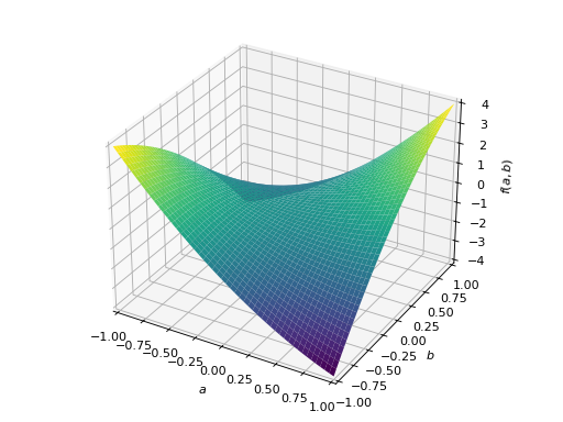
An example of non-symmetric positive definite matrix.
>>> A = Matrix([[1, 2], [-2, 1]]) >>> A.is_positive_definite True >>> A.is_positive_semidefinite True
>>> p = plot3d((x.T*A*x)[0, 0], (a, -1, 1), (b, -1, 1))

Notes
Although some people trivialize the definition of positive definite matrices only for symmetric or hermitian matrices, this restriction is not correct because it does not classify all instances of positive definite matrices from the definition \(x^T A x > 0\) or \(\text{re}(x^H A x) > 0\).
For instance,
Matrix([[1, 2], [-2, 1]])presented in the example above is an example of real positive definite matrix that is not symmetric.However, since the following formula holds true;
\[\text{re}(x^H A x) > 0 \iff \text{re}(x^H \frac{A + A^H}{2} x) > 0\]We can classify all positive definite matrices that may or may not be symmetric or hermitian by transforming the matrix to \(\frac{A + A^T}{2}\) or \(\frac{A + A^H}{2}\) (which is guaranteed to be always real symmetric or complex hermitian) and we can defer most of the studies to symmetric or hermitian positive definite matrices.
But it is a different problem for the existence of Cholesky decomposition. Because even though a non symmetric or a non hermitian matrix can be positive definite, Cholesky or LDL decomposition does not exist because the decompositions require the matrix to be symmetric or hermitian.
References
[R622]Johnson, C. R. “Positive Definite Matrices.” Amer. Math. Monthly 77, 259-264 1970.
- property is_negative_semidefinite
Finds out the definiteness of a matrix.
Explanation
A square real matrix \(A\) is:
A positive definite matrix if \(x^T A x > 0\) for all non-zero real vectors \(x\).
A positive semidefinite matrix if \(x^T A x \geq 0\) for all non-zero real vectors \(x\).
A negative definite matrix if \(x^T A x < 0\) for all non-zero real vectors \(x\).
A negative semidefinite matrix if \(x^T A x \leq 0\) for all non-zero real vectors \(x\).
An indefinite matrix if there exists non-zero real vectors \(x, y\) with \(x^T A x > 0 > y^T A y\).
A square complex matrix \(A\) is:
A positive definite matrix if \(\text{re}(x^H A x) > 0\) for all non-zero complex vectors \(x\).
A positive semidefinite matrix if \(\text{re}(x^H A x) \geq 0\) for all non-zero complex vectors \(x\).
A negative definite matrix if \(\text{re}(x^H A x) < 0\) for all non-zero complex vectors \(x\).
A negative semidefinite matrix if \(\text{re}(x^H A x) \leq 0\) for all non-zero complex vectors \(x\).
An indefinite matrix if there exists non-zero complex vectors \(x, y\) with \(\text{re}(x^H A x) > 0 > \text{re}(y^H A y)\).
A matrix need not be symmetric or hermitian to be positive definite.
A real non-symmetric matrix is positive definite if and only if \(\frac{A + A^T}{2}\) is positive definite.
A complex non-hermitian matrix is positive definite if and only if \(\frac{A + A^H}{2}\) is positive definite.
And this extension can apply for all the definitions above.
However, for complex cases, you can restrict the definition of \(\text{re}(x^H A x) > 0\) to \(x^H A x > 0\) and require the matrix to be hermitian. But we do not present this restriction for computation because you can check
M.is_hermitianindependently with this and use the same procedure.Examples
An example of symmetric positive definite matrix:
>>> from sympy import Matrix, symbols >>> from sympy.plotting import plot3d >>> a, b = symbols('a b') >>> x = Matrix([a, b])
>>> A = Matrix([[1, 0], [0, 1]]) >>> A.is_positive_definite True >>> A.is_positive_semidefinite True
>>> p = plot3d((x.T*A*x)[0, 0], (a, -1, 1), (b, -1, 1))

An example of symmetric positive semidefinite matrix:
>>> A = Matrix([[1, -1], [-1, 1]]) >>> A.is_positive_definite False >>> A.is_positive_semidefinite True
>>> p = plot3d((x.T*A*x)[0, 0], (a, -1, 1), (b, -1, 1))
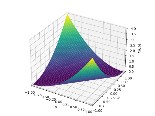
An example of symmetric negative definite matrix:
>>> A = Matrix([[-1, 0], [0, -1]]) >>> A.is_negative_definite True >>> A.is_negative_semidefinite True >>> A.is_indefinite False
>>> p = plot3d((x.T*A*x)[0, 0], (a, -1, 1), (b, -1, 1))

An example of symmetric indefinite matrix:
>>> A = Matrix([[1, 2], [2, -1]]) >>> A.is_indefinite True
>>> p = plot3d((x.T*A*x)[0, 0], (a, -1, 1), (b, -1, 1))

An example of non-symmetric positive definite matrix.
>>> A = Matrix([[1, 2], [-2, 1]]) >>> A.is_positive_definite True >>> A.is_positive_semidefinite True
>>> p = plot3d((x.T*A*x)[0, 0], (a, -1, 1), (b, -1, 1))

Notes
Although some people trivialize the definition of positive definite matrices only for symmetric or hermitian matrices, this restriction is not correct because it does not classify all instances of positive definite matrices from the definition \(x^T A x > 0\) or \(\text{re}(x^H A x) > 0\).
For instance,
Matrix([[1, 2], [-2, 1]])presented in the example above is an example of real positive definite matrix that is not symmetric.However, since the following formula holds true;
\[\text{re}(x^H A x) > 0 \iff \text{re}(x^H \frac{A + A^H}{2} x) > 0\]We can classify all positive definite matrices that may or may not be symmetric or hermitian by transforming the matrix to \(\frac{A + A^T}{2}\) or \(\frac{A + A^H}{2}\) (which is guaranteed to be always real symmetric or complex hermitian) and we can defer most of the studies to symmetric or hermitian positive definite matrices.
But it is a different problem for the existence of Cholesky decomposition. Because even though a non symmetric or a non hermitian matrix can be positive definite, Cholesky or LDL decomposition does not exist because the decompositions require the matrix to be symmetric or hermitian.
References
[R625]Johnson, C. R. “Positive Definite Matrices.” Amer. Math. Monthly 77, 259-264 1970.
- is_nilpotent()[source]
Checks if a matrix is nilpotent.
A matrix B is nilpotent if for some integer k, B**k is a zero matrix.
Examples
>>> from sympy import Matrix >>> a = Matrix([[0, 0, 0], [1, 0, 0], [1, 1, 0]]) >>> a.is_nilpotent() True
>>> a = Matrix([[1, 0, 1], [1, 0, 0], [1, 1, 0]]) >>> a.is_nilpotent() False
- property is_positive_definite
Finds out the definiteness of a matrix.
Explanation
A square real matrix \(A\) is:
A positive definite matrix if \(x^T A x > 0\) for all non-zero real vectors \(x\).
A positive semidefinite matrix if \(x^T A x \geq 0\) for all non-zero real vectors \(x\).
A negative definite matrix if \(x^T A x < 0\) for all non-zero real vectors \(x\).
A negative semidefinite matrix if \(x^T A x \leq 0\) for all non-zero real vectors \(x\).
An indefinite matrix if there exists non-zero real vectors \(x, y\) with \(x^T A x > 0 > y^T A y\).
A square complex matrix \(A\) is:
A positive definite matrix if \(\text{re}(x^H A x) > 0\) for all non-zero complex vectors \(x\).
A positive semidefinite matrix if \(\text{re}(x^H A x) \geq 0\) for all non-zero complex vectors \(x\).
A negative definite matrix if \(\text{re}(x^H A x) < 0\) for all non-zero complex vectors \(x\).
A negative semidefinite matrix if \(\text{re}(x^H A x) \leq 0\) for all non-zero complex vectors \(x\).
An indefinite matrix if there exists non-zero complex vectors \(x, y\) with \(\text{re}(x^H A x) > 0 > \text{re}(y^H A y)\).
A matrix need not be symmetric or hermitian to be positive definite.
A real non-symmetric matrix is positive definite if and only if \(\frac{A + A^T}{2}\) is positive definite.
A complex non-hermitian matrix is positive definite if and only if \(\frac{A + A^H}{2}\) is positive definite.
And this extension can apply for all the definitions above.
However, for complex cases, you can restrict the definition of \(\text{re}(x^H A x) > 0\) to \(x^H A x > 0\) and require the matrix to be hermitian. But we do not present this restriction for computation because you can check
M.is_hermitianindependently with this and use the same procedure.Examples
An example of symmetric positive definite matrix:
>>> from sympy import Matrix, symbols >>> from sympy.plotting import plot3d >>> a, b = symbols('a b') >>> x = Matrix([a, b])
>>> A = Matrix([[1, 0], [0, 1]]) >>> A.is_positive_definite True >>> A.is_positive_semidefinite True
>>> p = plot3d((x.T*A*x)[0, 0], (a, -1, 1), (b, -1, 1))
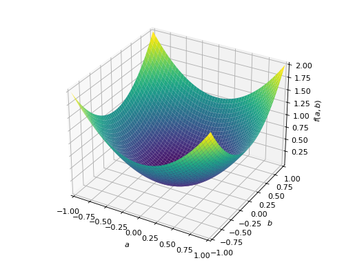
An example of symmetric positive semidefinite matrix:
>>> A = Matrix([[1, -1], [-1, 1]]) >>> A.is_positive_definite False >>> A.is_positive_semidefinite True
>>> p = plot3d((x.T*A*x)[0, 0], (a, -1, 1), (b, -1, 1))

An example of symmetric negative definite matrix:
>>> A = Matrix([[-1, 0], [0, -1]]) >>> A.is_negative_definite True >>> A.is_negative_semidefinite True >>> A.is_indefinite False
>>> p = plot3d((x.T*A*x)[0, 0], (a, -1, 1), (b, -1, 1))
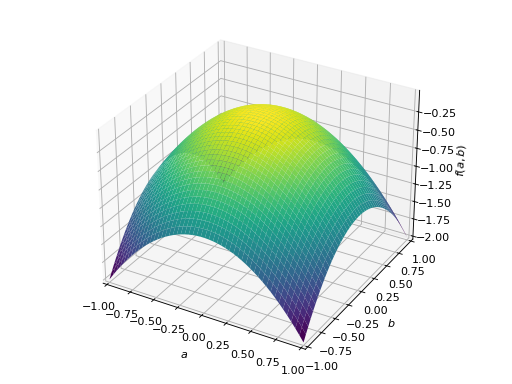
An example of symmetric indefinite matrix:
>>> A = Matrix([[1, 2], [2, -1]]) >>> A.is_indefinite True
>>> p = plot3d((x.T*A*x)[0, 0], (a, -1, 1), (b, -1, 1))

An example of non-symmetric positive definite matrix.
>>> A = Matrix([[1, 2], [-2, 1]]) >>> A.is_positive_definite True >>> A.is_positive_semidefinite True
>>> p = plot3d((x.T*A*x)[0, 0], (a, -1, 1), (b, -1, 1))

Notes
Although some people trivialize the definition of positive definite matrices only for symmetric or hermitian matrices, this restriction is not correct because it does not classify all instances of positive definite matrices from the definition \(x^T A x > 0\) or \(\text{re}(x^H A x) > 0\).
For instance,
Matrix([[1, 2], [-2, 1]])presented in the example above is an example of real positive definite matrix that is not symmetric.However, since the following formula holds true;
\[\text{re}(x^H A x) > 0 \iff \text{re}(x^H \frac{A + A^H}{2} x) > 0\]We can classify all positive definite matrices that may or may not be symmetric or hermitian by transforming the matrix to \(\frac{A + A^T}{2}\) or \(\frac{A + A^H}{2}\) (which is guaranteed to be always real symmetric or complex hermitian) and we can defer most of the studies to symmetric or hermitian positive definite matrices.
But it is a different problem for the existence of Cholesky decomposition. Because even though a non symmetric or a non hermitian matrix can be positive definite, Cholesky or LDL decomposition does not exist because the decompositions require the matrix to be symmetric or hermitian.
References
[R628]Johnson, C. R. “Positive Definite Matrices.” Amer. Math. Monthly 77, 259-264 1970.
- property is_positive_semidefinite
Finds out the definiteness of a matrix.
Explanation
A square real matrix \(A\) is:
A positive definite matrix if \(x^T A x > 0\) for all non-zero real vectors \(x\).
A positive semidefinite matrix if \(x^T A x \geq 0\) for all non-zero real vectors \(x\).
A negative definite matrix if \(x^T A x < 0\) for all non-zero real vectors \(x\).
A negative semidefinite matrix if \(x^T A x \leq 0\) for all non-zero real vectors \(x\).
An indefinite matrix if there exists non-zero real vectors \(x, y\) with \(x^T A x > 0 > y^T A y\).
A square complex matrix \(A\) is:
A positive definite matrix if \(\text{re}(x^H A x) > 0\) for all non-zero complex vectors \(x\).
A positive semidefinite matrix if \(\text{re}(x^H A x) \geq 0\) for all non-zero complex vectors \(x\).
A negative definite matrix if \(\text{re}(x^H A x) < 0\) for all non-zero complex vectors \(x\).
A negative semidefinite matrix if \(\text{re}(x^H A x) \leq 0\) for all non-zero complex vectors \(x\).
An indefinite matrix if there exists non-zero complex vectors \(x, y\) with \(\text{re}(x^H A x) > 0 > \text{re}(y^H A y)\).
A matrix need not be symmetric or hermitian to be positive definite.
A real non-symmetric matrix is positive definite if and only if \(\frac{A + A^T}{2}\) is positive definite.
A complex non-hermitian matrix is positive definite if and only if \(\frac{A + A^H}{2}\) is positive definite.
And this extension can apply for all the definitions above.
However, for complex cases, you can restrict the definition of \(\text{re}(x^H A x) > 0\) to \(x^H A x > 0\) and require the matrix to be hermitian. But we do not present this restriction for computation because you can check
M.is_hermitianindependently with this and use the same procedure.Examples
An example of symmetric positive definite matrix:
>>> from sympy import Matrix, symbols >>> from sympy.plotting import plot3d >>> a, b = symbols('a b') >>> x = Matrix([a, b])
>>> A = Matrix([[1, 0], [0, 1]]) >>> A.is_positive_definite True >>> A.is_positive_semidefinite True
>>> p = plot3d((x.T*A*x)[0, 0], (a, -1, 1), (b, -1, 1))

An example of symmetric positive semidefinite matrix:
>>> A = Matrix([[1, -1], [-1, 1]]) >>> A.is_positive_definite False >>> A.is_positive_semidefinite True
>>> p = plot3d((x.T*A*x)[0, 0], (a, -1, 1), (b, -1, 1))

An example of symmetric negative definite matrix:
>>> A = Matrix([[-1, 0], [0, -1]]) >>> A.is_negative_definite True >>> A.is_negative_semidefinite True >>> A.is_indefinite False
>>> p = plot3d((x.T*A*x)[0, 0], (a, -1, 1), (b, -1, 1))

An example of symmetric indefinite matrix:
>>> A = Matrix([[1, 2], [2, -1]]) >>> A.is_indefinite True
>>> p = plot3d((x.T*A*x)[0, 0], (a, -1, 1), (b, -1, 1))

An example of non-symmetric positive definite matrix.
>>> A = Matrix([[1, 2], [-2, 1]]) >>> A.is_positive_definite True >>> A.is_positive_semidefinite True
>>> p = plot3d((x.T*A*x)[0, 0], (a, -1, 1), (b, -1, 1))

Notes
Although some people trivialize the definition of positive definite matrices only for symmetric or hermitian matrices, this restriction is not correct because it does not classify all instances of positive definite matrices from the definition \(x^T A x > 0\) or \(\text{re}(x^H A x) > 0\).
For instance,
Matrix([[1, 2], [-2, 1]])presented in the example above is an example of real positive definite matrix that is not symmetric.However, since the following formula holds true;
\[\text{re}(x^H A x) > 0 \iff \text{re}(x^H \frac{A + A^H}{2} x) > 0\]We can classify all positive definite matrices that may or may not be symmetric or hermitian by transforming the matrix to \(\frac{A + A^T}{2}\) or \(\frac{A + A^H}{2}\) (which is guaranteed to be always real symmetric or complex hermitian) and we can defer most of the studies to symmetric or hermitian positive definite matrices.
But it is a different problem for the existence of Cholesky decomposition. Because even though a non symmetric or a non hermitian matrix can be positive definite, Cholesky or LDL decomposition does not exist because the decompositions require the matrix to be symmetric or hermitian.
References
[R631]Johnson, C. R. “Positive Definite Matrices.” Amer. Math. Monthly 77, 259-264 1970.
- property is_square
Checks if a matrix is square.
A matrix is square if the number of rows equals the number of columns. The empty matrix is square by definition, since the number of rows and the number of columns are both zero.
Examples
>>> from sympy import Matrix >>> a = Matrix([[1, 2, 3], [4, 5, 6]]) >>> b = Matrix([[1, 2, 3], [4, 5, 6], [7, 8, 9]]) >>> c = Matrix([]) >>> a.is_square False >>> b.is_square True >>> c.is_square True
- property is_strongly_diagonally_dominant
Tests if the matrix is row strongly diagonally dominant.
Explanation
A \(n, n\) matrix \(A\) is row strongly diagonally dominant if
\[\left|A_{i, i}\right| > \sum_{j = 0, j \neq i}^{n-1} \left|A_{i, j}\right| \quad {\text{for all }} i \in \{ 0, ..., n-1 \}\]Examples
>>> from sympy import Matrix >>> A = Matrix([[3, -2, 1], [1, -3, 2], [-1, 2, 4]]) >>> A.is_strongly_diagonally_dominant False
>>> A = Matrix([[-2, 2, 1], [1, 3, 2], [1, -2, 0]]) >>> A.is_strongly_diagonally_dominant False
>>> A = Matrix([[-4, 2, 1], [1, 6, 2], [1, -2, 5]]) >>> A.is_strongly_diagonally_dominant True
Notes
If you want to test whether a matrix is column diagonally dominant, you can apply the test after transposing the matrix.
- is_symbolic()[source]
Checks if any elements contain Symbols.
Examples
>>> from sympy import Matrix >>> from sympy.abc import x, y >>> M = Matrix([[x, y], [1, 0]]) >>> M.is_symbolic() True
- is_symmetric(simplify=True)[source]
Check if matrix is symmetric matrix, that is square matrix and is equal to its transpose.
By default, simplifications occur before testing symmetry. They can be skipped using ‘simplify=False’; while speeding things a bit, this may however induce false negatives.
Examples
>>> from sympy import Matrix >>> m = Matrix(2, 2, [0, 1, 1, 2]) >>> m Matrix([ [0, 1], [1, 2]]) >>> m.is_symmetric() True
>>> m = Matrix(2, 2, [0, 1, 2, 0]) >>> m Matrix([ [0, 1], [2, 0]]) >>> m.is_symmetric() False
>>> m = Matrix(2, 3, [0, 0, 0, 0, 0, 0]) >>> m Matrix([ [0, 0, 0], [0, 0, 0]]) >>> m.is_symmetric() False
>>> from sympy.abc import x, y >>> m = Matrix(3, 3, [1, x**2 + 2*x + 1, y, (x + 1)**2, 2, 0, y, 0, 3]) >>> m Matrix([ [ 1, x**2 + 2*x + 1, y], [(x + 1)**2, 2, 0], [ y, 0, 3]]) >>> m.is_symmetric() True
If the matrix is already simplified, you may speed-up is_symmetric() test by using ‘simplify=False’.
>>> bool(m.is_symmetric(simplify=False)) False >>> m1 = m.expand() >>> m1.is_symmetric(simplify=False) True
- property is_upper
Check if matrix is an upper triangular matrix. True can be returned even if the matrix is not square.
Examples
>>> from sympy import Matrix >>> m = Matrix(2, 2, [1, 0, 0, 1]) >>> m Matrix([ [1, 0], [0, 1]]) >>> m.is_upper True
>>> m = Matrix(4, 3, [5, 1, 9, 0, 4, 6, 0, 0, 5, 0, 0, 0]) >>> m Matrix([ [5, 1, 9], [0, 4, 6], [0, 0, 5], [0, 0, 0]]) >>> m.is_upper True
>>> m = Matrix(2, 3, [4, 2, 5, 6, 1, 1]) >>> m Matrix([ [4, 2, 5], [6, 1, 1]]) >>> m.is_upper False
See also
- property is_upper_hessenberg
Checks if the matrix is the upper-Hessenberg form.
The upper hessenberg matrix has zero entries below the first subdiagonal.
Examples
>>> from sympy import Matrix >>> a = Matrix([[1, 4, 2, 3], [3, 4, 1, 7], [0, 2, 3, 4], [0, 0, 1, 3]]) >>> a Matrix([ [1, 4, 2, 3], [3, 4, 1, 7], [0, 2, 3, 4], [0, 0, 1, 3]]) >>> a.is_upper_hessenberg True
See also
- property is_weakly_diagonally_dominant
Tests if the matrix is row weakly diagonally dominant.
Explanation
A \(n, n\) matrix \(A\) is row weakly diagonally dominant if
\[\left|A_{i, i}\right| \ge \sum_{j = 0, j \neq i}^{n-1} \left|A_{i, j}\right| \quad {\text{for all }} i \in \{ 0, ..., n-1 \}\]Examples
>>> from sympy import Matrix >>> A = Matrix([[3, -2, 1], [1, -3, 2], [-1, 2, 4]]) >>> A.is_weakly_diagonally_dominant True
>>> A = Matrix([[-2, 2, 1], [1, 3, 2], [1, -2, 0]]) >>> A.is_weakly_diagonally_dominant False
>>> A = Matrix([[-4, 2, 1], [1, 6, 2], [1, -2, 5]]) >>> A.is_weakly_diagonally_dominant True
Notes
If you want to test whether a matrix is column diagonally dominant, you can apply the test after transposing the matrix.
- property is_zero_matrix
Checks if a matrix is a zero matrix.
A matrix is zero if every element is zero. A matrix need not be square to be considered zero. The empty matrix is zero by the principle of vacuous truth. For a matrix that may or may not be zero (e.g. contains a symbol), this will be None
Examples
>>> from sympy import Matrix, zeros >>> from sympy.abc import x >>> a = Matrix([[0, 0], [0, 0]]) >>> b = zeros(3, 4) >>> c = Matrix([[0, 1], [0, 0]]) >>> d = Matrix([]) >>> e = Matrix([[x, 0], [0, 0]]) >>> a.is_zero_matrix True >>> b.is_zero_matrix True >>> c.is_zero_matrix False >>> d.is_zero_matrix True >>> e.is_zero_matrix
- iter_items()[source]
Iterate over indices and values of nonzero items.
Examples
>>> from sympy import Matrix >>> m = Matrix([[0, 1], [2, 3]]) >>> list(m.iter_items()) [((0, 1), 1), ((1, 0), 2), ((1, 1), 3)]
See also
- iter_values()[source]
Iterate over non-zero values of self.
Examples
>>> from sympy import Matrix >>> m = Matrix([[0, 1], [2, 3]]) >>> list(m.iter_values()) [1, 2, 3]
See also
- jacobian(X)[source]
Calculates the Jacobian matrix (derivative of a vector-valued function).
- Parameters:
``self`` : vector of expressions representing functions f_i(x_1, …, x_n).
X : set of x_i’s in order, it can be a list or a Matrix
Both ``self`` and X can be a row or a column matrix in any order
(i.e., jacobian() should always work).
Examples
>>> from sympy import sin, cos, Matrix >>> from sympy.abc import rho, phi >>> X = Matrix([rho*cos(phi), rho*sin(phi), rho**2]) >>> Y = Matrix([rho, phi]) >>> X.jacobian(Y) Matrix([ [cos(phi), -rho*sin(phi)], [sin(phi), rho*cos(phi)], [ 2*rho, 0]]) >>> X = Matrix([rho*cos(phi), rho*sin(phi)]) >>> X.jacobian(Y) Matrix([ [cos(phi), -rho*sin(phi)], [sin(phi), rho*cos(phi)]])
- classmethod jordan_block(
- size=None,
- eigenvalue=None,
- *,
- band='upper',
- **kwargs,
Returns a Jordan block
- Parameters:
size : Integer, optional
Specifies the shape of the Jordan block matrix.
eigenvalue : Number or Symbol
Specifies the value for the main diagonal of the matrix.
Note
The keyword
eigenvalis also specified as an alias of this keyword, but it is not recommended to use.We may deprecate the alias in later release.
band : ‘upper’ or ‘lower’, optional
Specifies the position of the off-diagonal to put \(1\) s on.
cls : Matrix, optional
Specifies the matrix class of the output form.
If it is not specified, the class type where the method is being executed on will be returned.
- Returns:
Matrix
A Jordan block matrix.
- Raises:
ValueError
If insufficient arguments are given for matrix size specification, or no eigenvalue is given.
Examples
Creating a default Jordan block:
>>> from sympy import Matrix >>> from sympy.abc import x >>> Matrix.jordan_block(4, x) Matrix([ [x, 1, 0, 0], [0, x, 1, 0], [0, 0, x, 1], [0, 0, 0, x]])
Creating an alternative Jordan block matrix where \(1\) is on lower off-diagonal:
>>> Matrix.jordan_block(4, x, band='lower') Matrix([ [x, 0, 0, 0], [1, x, 0, 0], [0, 1, x, 0], [0, 0, 1, x]])
Creating a Jordan block with keyword arguments
>>> Matrix.jordan_block(size=4, eigenvalue=x) Matrix([ [x, 1, 0, 0], [0, x, 1, 0], [0, 0, x, 1], [0, 0, 0, x]])
References
- jordan_form(
- calc_transform=True,
- **kwargs,
Return \((P, J)\) where \(J\) is a Jordan block matrix and \(P\) is a matrix such that \(M = P J P^{-1}\)
- Parameters:
calc_transform : bool
If
False, then only \(J\) is returned.chop : bool
All matrices are converted to exact types when computing eigenvalues and eigenvectors. As a result, there may be approximation errors. If
chop==True, these errors will be truncated.
Examples
>>> from sympy import Matrix >>> M = Matrix([[ 6, 5, -2, -3], [-3, -1, 3, 3], [ 2, 1, -2, -3], [-1, 1, 5, 5]]) >>> P, J = M.jordan_form() >>> J Matrix([ [2, 1, 0, 0], [0, 2, 0, 0], [0, 0, 2, 1], [0, 0, 0, 2]])
See also
- key2bounds(keys)[source]
Converts a key with potentially mixed types of keys (integer and slice) into a tuple of ranges and raises an error if any index is out of
self’s range.See also
- key2ij(key)[source]
Converts key into canonical form, converting integers or indexable items into valid integers for
self’s range or returning slices unchanged.See also
- left_eigenvects(**flags)[source]
Returns left eigenvectors and eigenvalues.
This function returns the list of triples (eigenval, multiplicity, basis) for the left eigenvectors. Options are the same as for eigenvects(), i.e. the
**flagsarguments gets passed directly to eigenvects().Examples
>>> from sympy import Matrix >>> M = Matrix([[0, 1, 1], [1, 0, 0], [1, 1, 1]]) >>> M.eigenvects() [(-1, 1, [Matrix([ [-1], [ 1], [ 0]])]), (0, 1, [Matrix([ [ 0], [-1], [ 1]])]), (2, 1, [Matrix([ [2/3], [1/3], [ 1]])])] >>> M.left_eigenvects() [(-1, 1, [Matrix([[-2, 1, 1]])]), (0, 1, [Matrix([[-1, -1, 1]])]), (2, 1, [Matrix([[1, 1, 1]])])]
- limit(*args)[source]
Calculate the limit of each element in the matrix.
argswill be passed to thelimitfunction.Examples
>>> from sympy import Matrix >>> from sympy.abc import x, y >>> M = Matrix([[x, y], [1, 0]]) >>> M.limit(x, 2) Matrix([ [2, y], [1, 0]])
- log(simplify=<function cancel>)[source]
Return the logarithm of a square matrix.
- Parameters:
simplify : function, bool
The function to simplify the result with.
Default is
cancel, which is effective to reduce the expression growing for taking reciprocals and inverses for symbolic matrices.
Examples
>>> from sympy import S, Matrix
Examples for positive-definite matrices:
>>> m = Matrix([[1, 1], [0, 1]]) >>> m.log() Matrix([ [0, 1], [0, 0]])
>>> m = Matrix([[S(5)/4, S(3)/4], [S(3)/4, S(5)/4]]) >>> m.log() Matrix([ [ 0, log(2)], [log(2), 0]])
Examples for non positive-definite matrices:
>>> m = Matrix([[S(3)/4, S(5)/4], [S(5)/4, S(3)/4]]) >>> m.log() Matrix([ [ I*pi/2, log(2) - I*pi/2], [log(2) - I*pi/2, I*pi/2]])
>>> m = Matrix( ... [[0, 0, 0, 1], ... [0, 0, 1, 0], ... [0, 1, 0, 0], ... [1, 0, 0, 0]]) >>> m.log() Matrix([ [ I*pi/2, 0, 0, -I*pi/2], [ 0, I*pi/2, -I*pi/2, 0], [ 0, -I*pi/2, I*pi/2, 0], [-I*pi/2, 0, 0, I*pi/2]])
- lower_triangular(k=0)[source]
Return the elements on and below the kth diagonal of a matrix. If k is not specified then simply returns lower-triangular portion of a matrix
Examples
>>> from sympy import ones >>> A = ones(4) >>> A.lower_triangular() Matrix([ [1, 0, 0, 0], [1, 1, 0, 0], [1, 1, 1, 0], [1, 1, 1, 1]])
>>> A.lower_triangular(-2) Matrix([ [0, 0, 0, 0], [0, 0, 0, 0], [1, 0, 0, 0], [1, 1, 0, 0]])
>>> A.lower_triangular(1) Matrix([ [1, 1, 0, 0], [1, 1, 1, 0], [1, 1, 1, 1], [1, 1, 1, 1]])
- minor(i, j, method='berkowitz')[source]
Return the (i,j) minor of
M. That is, return the determinant of the matrix obtained by deleting the \(i`th row and `j`th column from ``M`\).- Parameters:
i, j : int
The row and column to exclude to obtain the submatrix.
method : string, optional
Method to use to find the determinant of the submatrix, can be “bareiss”, “berkowitz”, “bird”, “laplace” or “lu”.
Examples
>>> from sympy import Matrix >>> M = Matrix([[1, 2, 3], [4, 5, 6], [7, 8, 9]]) >>> M.minor(1, 1) -12
See also
- minor_submatrix(i, j)[source]
Return the submatrix obtained by removing the \(i`th row and `j`th column from ``M`\) (works with Pythonic negative indices).
- Parameters:
i, j : int
The row and column to exclude to obtain the submatrix.
Examples
>>> from sympy import Matrix >>> M = Matrix([[1, 2, 3], [4, 5, 6], [7, 8, 9]]) >>> M.minor_submatrix(1, 1) Matrix([ [1, 3], [7, 9]])
- multiply(other, dotprodsimp=None)[source]
Same as __mul__() but with optional simplification.
- Parameters:
dotprodsimp : bool, optional
Specifies whether intermediate term algebraic simplification is used during matrix multiplications to control expression blowup and thus speed up calculation. Default is off.
- multiply_elementwise(other)[source]
Return the Hadamard product (elementwise product) of A and B
Examples
>>> from sympy import Matrix >>> A = Matrix([[0, 1, 2], [3, 4, 5]]) >>> B = Matrix([[1, 10, 100], [100, 10, 1]]) >>> A.multiply_elementwise(B) Matrix([ [ 0, 10, 200], [300, 40, 5]])
- norm(ord=None)[source]
Return the Norm of a Matrix or Vector.
In the simplest case this is the geometric size of the vector Other norms can be specified by the ord parameter
ord
norm for matrices
norm for vectors
None
Frobenius norm
2-norm
‘fro’
Frobenius norm
does not exist
inf
maximum row sum
max(abs(x))
-inf
–
min(abs(x))
1
maximum column sum
as below
-1
–
as below
2
2-norm (largest sing. value)
as below
-2
smallest singular value
as below
other
does not exist
sum(abs(x)**ord)**(1./ord)
Examples
>>> from sympy import Matrix, Symbol, trigsimp, cos, sin, oo >>> x = Symbol('x', real=True) >>> v = Matrix([cos(x), sin(x)]) >>> trigsimp( v.norm() ) 1 >>> v.norm(10) (sin(x)**10 + cos(x)**10)**(1/10) >>> A = Matrix([[1, 1], [1, 1]]) >>> A.norm(1) # maximum sum of absolute values of A is 2 2 >>> A.norm(2) # Spectral norm (max of |Ax|/|x| under 2-vector-norm) 2 >>> A.norm(-2) # Inverse spectral norm (smallest singular value) 0 >>> A.norm() # Frobenius Norm 2 >>> A.norm(oo) # Infinity Norm 2 >>> Matrix([1, -2]).norm(oo) 2 >>> Matrix([-1, 2]).norm(-oo) 1
See also
- normalized(
- iszerofunc=<function _iszero>,
Return the normalized version of
self.- Parameters:
iszerofunc : Function, optional
A function to determine whether
selfis a zero vector. The default_iszerotests to see if each element is exactly zero.- Returns:
Matrix
Normalized vector form of
self. It has the same length as a unit vector. However, a zero vector will be returned for a vector with norm 0.- Raises:
ShapeError
If the matrix is not in a vector form.
See also
- nullspace(
- simplify=False,
- iszerofunc=<function _iszero>,
Returns list of vectors (Matrix objects) that span nullspace of
MExamples
>>> from sympy import Matrix >>> M = Matrix(3, 3, [1, 3, 0, -2, -6, 0, 3, 9, 6]) >>> M Matrix([ [ 1, 3, 0], [-2, -6, 0], [ 3, 9, 6]]) >>> M.nullspace() [Matrix([ [-3], [ 1], [ 0]])]
See also
- classmethod ones(rows, cols=None, **kwargs)[source]
Returns a matrix of ones.
- Parameters:
rows : rows of the matrix
cols : cols of the matrix (if None, cols=rows)
Kwargs
cls : class of the returned matrix
- classmethod orthogonalize(*vecs, **kwargs)[source]
Apply the Gram-Schmidt orthogonalization procedure to vectors supplied in
vecs.- Parameters:
vecs
vectors to be made orthogonal
normalize : bool
If
True, return an orthonormal basis.rankcheck : bool
If
True, the computation does not stop when encountering linearly dependent vectors.If
False, it will raiseValueErrorwhen any zero or linearly dependent vectors are found.- Returns:
list
List of orthogonal (or orthonormal) basis vectors.
Examples
>>> from sympy import I, Matrix >>> v = [Matrix([1, I]), Matrix([1, -I])] >>> Matrix.orthogonalize(*v) [Matrix([ [1], [I]]), Matrix([ [ 1], [-I]])]
See also
References
- per()[source]
Returns the permanent of a matrix. Unlike determinant, permanent is defined for both square and non-square matrices.
For an m x n matrix, with m less than or equal to n, it is given as the sum over the permutations s of size less than or equal to m on [1, 2, … n] of the product from i = 1 to m of M[i, s[i]]. Taking the transpose will not affect the value of the permanent.
In the case of a square matrix, this is the same as the permutation definition of the determinant, but it does not take the sign of the permutation into account. Computing the permanent with this definition is quite inefficient, so here the Ryser formula is used.
Examples
>>> from sympy import Matrix >>> M = Matrix([[1, 2, 3], [4, 5, 6], [7, 8, 9]]) >>> M.per() 450 >>> M = Matrix([1, 5, 7]) >>> M.per() 13
References
[R634]Prof. Frank Ben’s notes: https://math.berkeley.edu/~bernd/ban275.pdf
[R635]Wikipedia article on Permanent: https://en.wikipedia.org/wiki/Permanent_%28mathematics%29
[R637]Permanent of a rectangular matrix : https://arxiv.org/pdf/0904.3251.pdf
- permute(
- perm,
- orientation='rows',
- direction='forward',
Permute the rows or columns of a matrix by the given list of swaps.
- Parameters:
perm : Permutation, list, or list of lists
A representation for the permutation.
If it is
Permutation, it is used directly with some resizing with respect to the matrix size.If it is specified as list of lists, (e.g.,
[[0, 1], [0, 2]]), then the permutation is formed from applying the product of cycles. The direction how the cyclic product is applied is described in below.If it is specified as a list, the list should represent an array form of a permutation. (e.g.,
[1, 2, 0]) which would would form the swapping function \(0 \mapsto 1, 1 \mapsto 2, 2\mapsto 0\).orientation : ‘rows’, ‘cols’
A flag to control whether to permute the rows or the columns
direction : ‘forward’, ‘backward’
A flag to control whether to apply the permutations from the start of the list first, or from the back of the list first.
For example, if the permutation specification is
[[0, 1], [0, 2]],If the flag is set to
'forward', the cycle would be formed as \(0 \mapsto 2, 2 \mapsto 1, 1 \mapsto 0\).If the flag is set to
'backward', the cycle would be formed as \(0 \mapsto 1, 1 \mapsto 2, 2 \mapsto 0\).If the argument
permis not in a form of list of lists, this flag takes no effect.
Examples
>>> from sympy import eye >>> M = eye(3) >>> M.permute([[0, 1], [0, 2]], orientation='rows', direction='forward') Matrix([ [0, 0, 1], [1, 0, 0], [0, 1, 0]])
>>> from sympy import eye >>> M = eye(3) >>> M.permute([[0, 1], [0, 2]], orientation='rows', direction='backward') Matrix([ [0, 1, 0], [0, 0, 1], [1, 0, 0]])
Notes
If a bijective function \(\sigma : \mathbb{N}_0 \rightarrow \mathbb{N}_0\) denotes the permutation.
If the matrix \(A\) is the matrix to permute, represented as a horizontal or a vertical stack of vectors:
\[\begin{split}A = \begin{bmatrix} a_0 \\ a_1 \\ \vdots \\ a_{n-1} \end{bmatrix} = \begin{bmatrix} \alpha_0 & \alpha_1 & \cdots & \alpha_{n-1} \end{bmatrix}\end{split}\]If the matrix \(B\) is the result, the permutation of matrix rows is defined as:
\[\begin{split}B := \begin{bmatrix} a_{\sigma(0)} \\ a_{\sigma(1)} \\ \vdots \\ a_{\sigma(n-1)} \end{bmatrix}\end{split}\]And the permutation of matrix columns is defined as:
\[B := \begin{bmatrix} \alpha_{\sigma(0)} & \alpha_{\sigma(1)} & \cdots & \alpha_{\sigma(n-1)} \end{bmatrix}\]
- permute_cols(
- swaps,
- direction='forward',
Alias for
self.permute(swaps, orientation='cols', direction=direction)See also
- permute_rows(
- swaps,
- direction='forward',
Alias for
self.permute(swaps, orientation='rows', direction=direction)See also
- pinv(method='RD')[source]
Calculate the Moore-Penrose pseudoinverse of the matrix.
The Moore-Penrose pseudoinverse exists and is unique for any matrix. If the matrix is invertible, the pseudoinverse is the same as the inverse.
- Parameters:
method : String, optional
Specifies the method for computing the pseudoinverse.
If
'RD', Rank-Decomposition will be used.If
'ED', Diagonalization will be used.
Examples
Computing pseudoinverse by rank decomposition :
>>> from sympy import Matrix >>> A = Matrix([[1, 2, 3], [4, 5, 6]]) >>> A.pinv() Matrix([ [-17/18, 4/9], [ -1/9, 1/9], [ 13/18, -2/9]])
Computing pseudoinverse by diagonalization :
>>> B = A.pinv(method='ED') >>> B.simplify() >>> B Matrix([ [-17/18, 4/9], [ -1/9, 1/9], [ 13/18, -2/9]])
See also
References
- pinv_solve(B, arbitrary_matrix=None)[source]
Solve
Ax = Busing the Moore-Penrose pseudoinverse.There may be zero, one, or infinite solutions. If one solution exists, it will be returned. If infinite solutions exist, one will be returned based on the value of arbitrary_matrix. If no solutions exist, the least-squares solution is returned.
- Parameters:
B : Matrix
The right hand side of the equation to be solved for. Must have the same number of rows as matrix A.
arbitrary_matrix : Matrix
If the system is underdetermined (e.g. A has more columns than rows), infinite solutions are possible, in terms of an arbitrary matrix. This parameter may be set to a specific matrix to use for that purpose; if so, it must be the same shape as x, with as many rows as matrix A has columns, and as many columns as matrix B. If left as None, an appropriate matrix containing dummy symbols in the form of
wn_mwill be used, with n and m being row and column position of each symbol.- Returns:
x : Matrix
The matrix that will satisfy
Ax = B. Will have as many rows as matrix A has columns, and as many columns as matrix B.
Examples
>>> from sympy import Matrix >>> A = Matrix([[1, 2, 3], [4, 5, 6]]) >>> B = Matrix([7, 8]) >>> A.pinv_solve(B) Matrix([ [ _w0_0/6 - _w1_0/3 + _w2_0/6 - 55/18], [-_w0_0/3 + 2*_w1_0/3 - _w2_0/3 + 1/9], [ _w0_0/6 - _w1_0/3 + _w2_0/6 + 59/18]]) >>> A.pinv_solve(B, arbitrary_matrix=Matrix([0, 0, 0])) Matrix([ [-55/18], [ 1/9], [ 59/18]])
Notes
This may return either exact solutions or least squares solutions. To determine which, check
A * A.pinv() * B == B. It will be True if exact solutions exist, and False if only a least-squares solution exists. Be aware that the left hand side of that equation may need to be simplified to correctly compare to the right hand side.See also
sympy.matrices.dense.DenseMatrix.lower_triangular_solve,sympy.matrices.dense.DenseMatrix.upper_triangular_solve,gauss_jordan_solve,cholesky_solve,diagonal_solve,LDLsolve,LUsolve,QRsolve,pinvReferences
- pow(exp, method=None)[source]
Return self**exp a scalar or symbol.
- Parameters:
method : multiply, mulsimp, jordan, cayley
If multiply then it returns exponentiation using recursion. If jordan then Jordan form exponentiation will be used. If cayley then the exponentiation is done using Cayley-Hamilton theorem. If mulsimp then the exponentiation is done using recursion with dotprodsimp. This specifies whether intermediate term algebraic simplification is used during naive matrix power to control expression blowup and thus speed up calculation. If None, then it heuristically decides which method to use.
- print_nonzero(symb='X')[source]
Shows location of non-zero entries for fast shape lookup.
Examples
>>> from sympy import Matrix, eye >>> m = Matrix(2, 3, lambda i, j: i*3+j) >>> m Matrix([ [0, 1, 2], [3, 4, 5]]) >>> m.print_nonzero() [ XX] [XXX] >>> m = eye(4) >>> m.print_nonzero("x") [x ] [ x ] [ x ] [ x]
- project(v)[source]
Return the projection of
selfonto the line containingv.Examples
>>> from sympy import Matrix, S, sqrt >>> V = Matrix([sqrt(3)/2, S.Half]) >>> x = Matrix([[1, 0]]) >>> V.project(x) Matrix([[sqrt(3)/2, 0]]) >>> V.project(-x) Matrix([[sqrt(3)/2, 0]])
- rank(
- iszerofunc=<function _iszero>,
- simplify=False,
Returns the rank of a matrix.
Examples
>>> from sympy import Matrix >>> from sympy.abc import x >>> m = Matrix([[1, 2], [x, 1 - 1/x]]) >>> m.rank() 2 >>> n = Matrix(3, 3, range(1, 10)) >>> n.rank() 2
- rank_decomposition(
- iszerofunc=<function _iszero>,
- simplify=False,
Returns a pair of matrices (\(C\), \(F\)) with matching rank such that \(A = C F\).
- Parameters:
iszerofunc : Function, optional
A function used for detecting whether an element can act as a pivot.
lambda x: x.is_zerois used by default.simplify : Bool or Function, optional
A function used to simplify elements when looking for a pivot. By default SymPy’s
simplifyis used.- Returns:
(C, F) : Matrices
\(C\) and \(F\) are full-rank matrices with rank as same as \(A\), whose product gives \(A\).
See Notes for additional mathematical details.
Examples
>>> from sympy import Matrix >>> A = Matrix([ ... [1, 3, 1, 4], ... [2, 7, 3, 9], ... [1, 5, 3, 1], ... [1, 2, 0, 8] ... ]) >>> C, F = A.rank_decomposition() >>> C Matrix([ [1, 3, 4], [2, 7, 9], [1, 5, 1], [1, 2, 8]]) >>> F Matrix([ [1, 0, -2, 0], [0, 1, 1, 0], [0, 0, 0, 1]]) >>> C * F == A True
Notes
Obtaining \(F\), an RREF of \(A\), is equivalent to creating a product
\[E_n E_{n-1} ... E_1 A = F\]where \(E_n, E_{n-1}, \dots, E_1\) are the elimination matrices or permutation matrices equivalent to each row-reduction step.
The inverse of the same product of elimination matrices gives \(C\):
\[C = \left(E_n E_{n-1} \dots E_1\right)^{-1}\]It is not necessary, however, to actually compute the inverse: the columns of \(C\) are those from the original matrix with the same column indices as the indices of the pivot columns of \(F\).
References
[R641]Piziak, R.; Odell, P. L. (1 June 1999). “Full Rank Factorization of Matrices”. Mathematics Magazine. 72 (3): 193. doi:10.2307/2690882
- refine(assumptions=True)[source]
Apply refine to each element of the matrix.
Examples
>>> from sympy import Symbol, Matrix, Abs, sqrt, Q >>> x = Symbol('x') >>> Matrix([[Abs(x)**2, sqrt(x**2)],[sqrt(x**2), Abs(x)**2]]) Matrix([ [ Abs(x)**2, sqrt(x**2)], [sqrt(x**2), Abs(x)**2]]) >>> _.refine(Q.real(x)) Matrix([ [ x**2, Abs(x)], [Abs(x), x**2]])
- replace(
- F,
- G,
- map=False,
- simultaneous=True,
- exact=None,
Replaces Function F in Matrix entries with Function G.
Examples
>>> from sympy import symbols, Function, Matrix >>> F, G = symbols('F, G', cls=Function) >>> M = Matrix(2, 2, lambda i, j: F(i+j)) ; M Matrix([ [F(0), F(1)], [F(1), F(2)]]) >>> N = M.replace(F,G) >>> N Matrix([ [G(0), G(1)], [G(1), G(2)]])
- reshape(rows, cols)[source]
Reshape the matrix. Total number of elements must remain the same.
Examples
>>> from sympy import Matrix >>> m = Matrix(2, 3, lambda i, j: 1) >>> m Matrix([ [1, 1, 1], [1, 1, 1]]) >>> m.reshape(1, 6) Matrix([[1, 1, 1, 1, 1, 1]]) >>> m.reshape(3, 2) Matrix([ [1, 1], [1, 1], [1, 1]])
- rmultiply(other, dotprodsimp=None)[source]
Same as __rmul__() but with optional simplification.
- Parameters:
dotprodsimp : bool, optional
Specifies whether intermediate term algebraic simplification is used during matrix multiplications to control expression blowup and thus speed up calculation. Default is off.
- rot90(k=1)[source]
Rotates Matrix by 90 degrees
- Parameters:
k : int
Specifies how many times the matrix is rotated by 90 degrees (clockwise when positive, counter-clockwise when negative).
Examples
>>> from sympy import Matrix, symbols >>> A = Matrix(2, 2, symbols('a:d')) >>> A Matrix([ [a, b], [c, d]])
Rotating the matrix clockwise one time:
>>> A.rot90(1) Matrix([ [c, a], [d, b]])
Rotating the matrix anticlockwise two times:
>>> A.rot90(-2) Matrix([ [d, c], [b, a]])
- row(i)[source]
Elementary row selector.
Examples
>>> from sympy import eye >>> eye(2).row(0) Matrix([[1, 0]])
See also
- row_insert(pos, other)[source]
Insert one or more rows at the given row position.
Examples
>>> from sympy import zeros, ones >>> M = zeros(3) >>> V = ones(1, 3) >>> M.row_insert(1, V) Matrix([ [0, 0, 0], [1, 1, 1], [0, 0, 0], [0, 0, 0]])
See also
- row_join(other)[source]
Concatenates two matrices along self’s last and rhs’s first column
Examples
>>> from sympy import zeros, ones >>> M = zeros(3) >>> V = ones(3, 1) >>> M.row_join(V) Matrix([ [0, 0, 0, 1], [0, 0, 0, 1], [0, 0, 0, 1]])
- rowspace(simplify=False)[source]
Returns a list of vectors that span the row space of
M.Examples
>>> from sympy import Matrix >>> M = Matrix(3, 3, [1, 3, 0, -2, -6, 0, 3, 9, 6]) >>> M Matrix([ [ 1, 3, 0], [-2, -6, 0], [ 3, 9, 6]]) >>> M.rowspace() [Matrix([[1, 3, 0]]), Matrix([[0, 0, 6]])]
- rref(
- iszerofunc=<function _iszero>,
- simplify=False,
- pivots=True,
- normalize_last=True,
Return reduced row-echelon form of matrix and indices of pivot vars.
- Parameters:
iszerofunc : Function
A function used for detecting whether an element can act as a pivot.
lambda x: x.is_zerois used by default.simplify : Function
A function used to simplify elements when looking for a pivot. By default SymPy’s
simplifyis used.pivots : True or False
If
True, a tuple containing the row-reduced matrix and a tuple of pivot columns is returned. IfFalsejust the row-reduced matrix is returned.normalize_last : True or False
If
True, no pivots are normalized to \(1\) until after all entries above and below each pivot are zeroed. This means the row reduction algorithm is fraction free until the very last step. IfFalse, the naive row reduction procedure is used where each pivot is normalized to be \(1\) before row operations are used to zero above and below the pivot.
Examples
>>> from sympy import Matrix >>> from sympy.abc import x >>> m = Matrix([[1, 2], [x, 1 - 1/x]]) >>> m.rref() (Matrix([ [1, 0], [0, 1]]), (0, 1)) >>> rref_matrix, rref_pivots = m.rref() >>> rref_matrix Matrix([ [1, 0], [0, 1]]) >>> rref_pivots (0, 1)
iszerofunccan correct rounding errors in matrices with float values. In the following example, callingrref()leads to floating point errors, incorrectly row reducing the matrix.iszerofunc= lambda x: abs(x) < 1e-9sets sufficiently small numbers to zero, avoiding this error.>>> m = Matrix([[0.9, -0.1, -0.2, 0], [-0.8, 0.9, -0.4, 0], [-0.1, -0.8, 0.6, 0]]) >>> m.rref() (Matrix([ [1, 0, 0, 0], [0, 1, 0, 0], [0, 0, 1, 0]]), (0, 1, 2)) >>> m.rref(iszerofunc=lambda x:abs(x)<1e-9) (Matrix([ [1, 0, -0.301369863013699, 0], [0, 1, -0.712328767123288, 0], [0, 0, 0, 0]]), (0, 1))
Notes
The default value of
normalize_last=Truecan provide significant speedup to row reduction, especially on matrices with symbols. However, if you depend on the form row reduction algorithm leaves entries of the matrix, setnormalize_last=False
- rref_rhs(rhs)[source]
Return reduced row-echelon form of matrix, matrix showing rhs after reduction steps.
rhsmust have the same number of rows asself.Examples
>>> from sympy import Matrix, symbols >>> r1, r2 = symbols('r1 r2') >>> Matrix([[1, 1], [2, 1]]).rref_rhs(Matrix([r1, r2])) (Matrix([ [1, 0], [0, 1]]), Matrix([ [ -r1 + r2], [2*r1 - r2]]))
- property shape
The shape (dimensions) of the matrix as the 2-tuple (rows, cols).
Examples
>>> from sympy import zeros >>> M = zeros(2, 3) >>> M.shape (2, 3) >>> M.rows 2 >>> M.cols 3
- simplify(**kwargs)[source]
Apply simplify to each element of the matrix.
Examples
>>> from sympy.abc import x, y >>> from sympy import SparseMatrix, sin, cos >>> SparseMatrix(1, 1, [x*sin(y)**2 + x*cos(y)**2]) Matrix([[x*sin(y)**2 + x*cos(y)**2]]) >>> _.simplify() Matrix([[x]])
- singular_value_decomposition()[source]
Returns a Condensed Singular Value decomposition.
Explanation
A Singular Value decomposition is a decomposition in the form \(A = U \Sigma V^H\) where
\(U, V\) are column orthogonal matrix.
\(\Sigma\) is a diagonal matrix, where the main diagonal contains singular values of matrix A.
A column orthogonal matrix satisfies \(\mathbb{I} = U^H U\) while a full orthogonal matrix satisfies relation \(\mathbb{I} = U U^H = U^H U\) where \(\mathbb{I}\) is an identity matrix with matching dimensions.
For matrices which are not square or are rank-deficient, it is sufficient to return a column orthogonal matrix because augmenting them may introduce redundant computations. In condensed Singular Value Decomposition we only return column orthogonal matrices because of this reason
If you want to augment the results to return a full orthogonal decomposition, you should use the following procedures.
Augment the \(U, V\) matrices with columns that are orthogonal to every other columns and make it square.
Augment the \(\Sigma\) matrix with zero rows to make it have the same shape as the original matrix.
The procedure will be illustrated in the examples section.
Examples
we take a full rank matrix first:
>>> from sympy import Matrix >>> A = Matrix([[1, 2],[2,1]]) >>> U, S, V = A.singular_value_decomposition() >>> U Matrix([ [ sqrt(2)/2, sqrt(2)/2], [-sqrt(2)/2, sqrt(2)/2]]) >>> S Matrix([ [1, 0], [0, 3]]) >>> V Matrix([ [-sqrt(2)/2, sqrt(2)/2], [ sqrt(2)/2, sqrt(2)/2]])
If a matrix if square and full rank both U, V are orthogonal in both directions
>>> U * U.H Matrix([ [1, 0], [0, 1]]) >>> U.H * U Matrix([ [1, 0], [0, 1]])
>>> V * V.H Matrix([ [1, 0], [0, 1]]) >>> V.H * V Matrix([ [1, 0], [0, 1]]) >>> A == U * S * V.H True
>>> C = Matrix([ ... [1, 0, 0, 0, 2], ... [0, 0, 3, 0, 0], ... [0, 0, 0, 0, 0], ... [0, 2, 0, 0, 0], ... ]) >>> U, S, V = C.singular_value_decomposition()
>>> V.H * V Matrix([ [1, 0, 0], [0, 1, 0], [0, 0, 1]]) >>> V * V.H Matrix([ [1/5, 0, 0, 0, 2/5], [ 0, 1, 0, 0, 0], [ 0, 0, 1, 0, 0], [ 0, 0, 0, 0, 0], [2/5, 0, 0, 0, 4/5]])
If you want to augment the results to be a full orthogonal decomposition, you should augment \(V\) with an another orthogonal column.
You are able to append an arbitrary standard basis that are linearly independent to every other columns and you can run the Gram-Schmidt process to make them augmented as orthogonal basis.
>>> V_aug = V.row_join(Matrix([[0,0,0,0,1], ... [0,0,0,1,0]]).H) >>> V_aug = V_aug.QRdecomposition()[0] >>> V_aug Matrix([ [0, sqrt(5)/5, 0, -2*sqrt(5)/5, 0], [1, 0, 0, 0, 0], [0, 0, 1, 0, 0], [0, 0, 0, 0, 1], [0, 2*sqrt(5)/5, 0, sqrt(5)/5, 0]]) >>> V_aug.H * V_aug Matrix([ [1, 0, 0, 0, 0], [0, 1, 0, 0, 0], [0, 0, 1, 0, 0], [0, 0, 0, 1, 0], [0, 0, 0, 0, 1]]) >>> V_aug * V_aug.H Matrix([ [1, 0, 0, 0, 0], [0, 1, 0, 0, 0], [0, 0, 1, 0, 0], [0, 0, 0, 1, 0], [0, 0, 0, 0, 1]])
Similarly we augment U
>>> U_aug = U.row_join(Matrix([0,0,1,0])) >>> U_aug = U_aug.QRdecomposition()[0] >>> U_aug Matrix([ [0, 1, 0, 0], [0, 0, 1, 0], [0, 0, 0, 1], [1, 0, 0, 0]])
>>> U_aug.H * U_aug Matrix([ [1, 0, 0, 0], [0, 1, 0, 0], [0, 0, 1, 0], [0, 0, 0, 1]]) >>> U_aug * U_aug.H Matrix([ [1, 0, 0, 0], [0, 1, 0, 0], [0, 0, 1, 0], [0, 0, 0, 1]])
We add 2 zero columns and one row to S
>>> S_aug = S.col_join(Matrix([[0,0,0]])) >>> S_aug = S_aug.row_join(Matrix([[0,0,0,0], ... [0,0,0,0]]).H) >>> S_aug Matrix([ [2, 0, 0, 0, 0], [0, sqrt(5), 0, 0, 0], [0, 0, 3, 0, 0], [0, 0, 0, 0, 0]])
>>> U_aug * S_aug * V_aug.H == C True
- singular_values()[source]
Compute the singular values of a Matrix
Examples
>>> from sympy import Matrix, Symbol >>> x = Symbol('x', real=True) >>> M = Matrix([[0, 1, 0], [0, x, 0], [-1, 0, 0]]) >>> M.singular_values() [sqrt(x**2 + 1), 1, 0]
See also
- solve(rhs, method='GJ')[source]
Solves linear equation where the unique solution exists.
- Parameters:
rhs : Matrix
Vector representing the right hand side of the linear equation.
method : string, optional
If set to
'GJ'or'GE', the Gauss-Jordan elimination will be used, which is implemented in the routinegauss_jordan_solve.If set to
'LU',LUsolveroutine will be used.If set to
'QR',QRsolveroutine will be used.If set to
'PINV',pinv_solveroutine will be used.If set to
'CRAMER',cramer_solveroutine will be used.It also supports the methods available for special linear systems
For positive definite systems:
If set to
'CH',cholesky_solveroutine will be used.If set to
'LDL',LDLsolveroutine will be used.To use a different method and to compute the solution via the inverse, use a method defined in the .inv() docstring.
- Returns:
solutions : Matrix
Vector representing the solution.
- Raises:
ValueError
If there is not a unique solution then a
ValueErrorwill be raised.If
Mis not square, aValueErrorand a different routine for solving the system will be suggested.
- solve_least_squares(rhs, method='CH')[source]
Return the least-square fit to the data.
- Parameters:
rhs : Matrix
Vector representing the right hand side of the linear equation.
method : string or boolean, optional
If set to
'CH',cholesky_solveroutine will be used.If set to
'LDL',LDLsolveroutine will be used.If set to
'QR',QRsolveroutine will be used.If set to
'PINV',pinv_solveroutine will be used.Otherwise, the conjugate of
Mwill be used to create a system of equations that is passed tosolvealong with the hint defined bymethod.- Returns:
solutions : Matrix
Vector representing the solution.
Examples
>>> from sympy import Matrix, ones >>> A = Matrix([1, 2, 3]) >>> B = Matrix([2, 3, 4]) >>> S = Matrix(A.row_join(B)) >>> S Matrix([ [1, 2], [2, 3], [3, 4]])
If each line of S represent coefficients of Ax + By and x and y are [2, 3] then S*xy is:
>>> r = S*Matrix([2, 3]); r Matrix([ [ 8], [13], [18]])
But let’s add 1 to the middle value and then solve for the least-squares value of xy:
>>> xy = S.solve_least_squares(Matrix([8, 14, 18])); xy Matrix([ [ 5/3], [10/3]])
The error is given by S*xy - r:
>>> S*xy - r Matrix([ [1/3], [1/3], [1/3]]) >>> _.norm().n(2) 0.58
If a different xy is used, the norm will be higher:
>>> xy += ones(2, 1)/10 >>> (S*xy - r).norm().n(2) 1.5
- strongly_connected_components()[source]
Returns the list of strongly connected vertices of the graph when a square matrix is viewed as a weighted graph.
Examples
>>> from sympy import Matrix >>> A = Matrix([ ... [44, 0, 0, 0, 43, 0, 45, 0, 0], ... [0, 66, 62, 61, 0, 68, 0, 60, 67], ... [0, 0, 22, 21, 0, 0, 0, 20, 0], ... [0, 0, 12, 11, 0, 0, 0, 10, 0], ... [34, 0, 0, 0, 33, 0, 35, 0, 0], ... [0, 86, 82, 81, 0, 88, 0, 80, 87], ... [54, 0, 0, 0, 53, 0, 55, 0, 0], ... [0, 0, 2, 1, 0, 0, 0, 0, 0], ... [0, 76, 72, 71, 0, 78, 0, 70, 77]]) >>> A.strongly_connected_components() [[0, 4, 6], [2, 3, 7], [1, 5, 8]]
- strongly_connected_components_decomposition(
- lower=True,
Decomposes a square matrix into block triangular form only using the permutations.
- Parameters:
lower : bool
Makes \(B\) lower block triangular when
True. Otherwise, makes \(B\) upper block triangular.- Returns:
P, B : PermutationMatrix, BlockMatrix
P is a permutation matrix for the similarity transform as in the explanation. And B is the block triangular matrix of the result of the permutation.
Explanation
The decomposition is in a form of \(A = P^{-1} B P\) where \(P\) is a permutation matrix and \(B\) is a block diagonal matrix.
Examples
>>> from sympy import Matrix, pprint >>> A = Matrix([ ... [44, 0, 0, 0, 43, 0, 45, 0, 0], ... [0, 66, 62, 61, 0, 68, 0, 60, 67], ... [0, 0, 22, 21, 0, 0, 0, 20, 0], ... [0, 0, 12, 11, 0, 0, 0, 10, 0], ... [34, 0, 0, 0, 33, 0, 35, 0, 0], ... [0, 86, 82, 81, 0, 88, 0, 80, 87], ... [54, 0, 0, 0, 53, 0, 55, 0, 0], ... [0, 0, 2, 1, 0, 0, 0, 0, 0], ... [0, 76, 72, 71, 0, 78, 0, 70, 77]])
A lower block triangular decomposition:
>>> P, B = A.strongly_connected_components_decomposition() >>> pprint(P) PermutationMatrix((8)(1 4 3 2 6)(5 7)) >>> pprint(B) [[44 43 45] [0 0 0] [0 0 0] ] [[ ] [ ] [ ] ] [[34 33 35] [0 0 0] [0 0 0] ] [[ ] [ ] [ ] ] [[54 53 55] [0 0 0] [0 0 0] ] [ ] [ [0 0 0] [22 21 20] [0 0 0] ] [ [ ] [ ] [ ] ] [ [0 0 0] [12 11 10] [0 0 0] ] [ [ ] [ ] [ ] ] [ [0 0 0] [2 1 0 ] [0 0 0] ] [ ] [ [0 0 0] [62 61 60] [66 68 67]] [ [ ] [ ] [ ]] [ [0 0 0] [82 81 80] [86 88 87]] [ [ ] [ ] [ ]] [ [0 0 0] [72 71 70] [76 78 77]]
>>> P = P.as_explicit() >>> B = B.as_explicit() >>> P.T * B * P == A True
An upper block triangular decomposition:
>>> P, B = A.strongly_connected_components_decomposition(lower=False) >>> pprint(P) PermutationMatrix((0 1 5 7 4 3 2 8 6)) >>> pprint(B) [[66 68 67] [62 61 60] [0 0 0] ] [[ ] [ ] [ ] ] [[86 88 87] [82 81 80] [0 0 0] ] [[ ] [ ] [ ] ] [[76 78 77] [72 71 70] [0 0 0] ] [ ] [ [0 0 0] [22 21 20] [0 0 0] ] [ [ ] [ ] [ ] ] [ [0 0 0] [12 11 10] [0 0 0] ] [ [ ] [ ] [ ] ] [ [0 0 0] [2 1 0 ] [0 0 0] ] [ ] [ [0 0 0] [0 0 0] [44 43 45]] [ [ ] [ ] [ ]] [ [0 0 0] [0 0 0] [34 33 35]] [ [ ] [ ] [ ]] [ [0 0 0] [0 0 0] [54 53 55]]
>>> P = P.as_explicit() >>> B = B.as_explicit() >>> P.T * B * P == A True
- subs(*args, **kwargs)[source]
Return a new matrix with subs applied to each entry.
Examples
>>> from sympy.abc import x, y >>> from sympy import SparseMatrix, Matrix >>> SparseMatrix(1, 1, [x]) Matrix([[x]]) >>> _.subs(x, y) Matrix([[y]]) >>> Matrix(_).subs(y, x) Matrix([[x]])
- table(
- printer,
- rowstart='[',
- rowend=']',
- rowsep='\n',
- colsep=', ',
- align='right',
String form of Matrix as a table.
printeris the printer to use for on the elements (generally something like StrPrinter())rowstartis the string used to start each row (by default ‘[‘).rowendis the string used to end each row (by default ‘]’).rowsepis the string used to separate rows (by default a newline).colsepis the string used to separate columns (by default ‘, ‘).aligndefines how the elements are aligned. Must be one of ‘left’, ‘right’, or ‘center’. You can also use ‘<’, ‘>’, and ‘^’ to mean the same thing, respectively.This is used by the string printer for Matrix.
Examples
>>> from sympy import Matrix, StrPrinter >>> M = Matrix([[1, 2], [-33, 4]]) >>> printer = StrPrinter() >>> M.table(printer) '[ 1, 2]\n[-33, 4]' >>> print(M.table(printer)) [ 1, 2] [-33, 4] >>> print(M.table(printer, rowsep=',\n')) [ 1, 2], [-33, 4] >>> print('[%s]' % M.table(printer, rowsep=',\n')) [[ 1, 2], [-33, 4]] >>> print(M.table(printer, colsep=' ')) [ 1 2] [-33 4] >>> print(M.table(printer, align='center')) [ 1 , 2] [-33, 4] >>> print(M.table(printer, rowstart='{', rowend='}')) { 1, 2} {-33, 4}
- todod()[source]
Returns matrix as dict of dicts containing non-zero elements of the Matrix
Examples
>>> from sympy import Matrix >>> A = Matrix([[0, 1],[0, 3]]) >>> A Matrix([ [0, 1], [0, 3]]) >>> A.todod() {0: {1: 1}, 1: {1: 3}}
- todok()[source]
Return the matrix as dictionary of keys.
Examples
>>> from sympy import Matrix >>> M = Matrix.eye(3) >>> M.todok() {(0, 0): 1, (1, 1): 1, (2, 2): 1}
- tolist()[source]
Return the Matrix as a nested Python list.
Examples
>>> from sympy import Matrix, ones >>> m = Matrix(3, 3, range(9)) >>> m Matrix([ [0, 1, 2], [3, 4, 5], [6, 7, 8]]) >>> m.tolist() [[0, 1, 2], [3, 4, 5], [6, 7, 8]] >>> ones(3, 0).tolist() [[], [], []]
When there are no rows then it will not be possible to tell how many columns were in the original matrix:
>>> ones(0, 3).tolist() []
- trace()[source]
Returns the trace of a square matrix i.e. the sum of the diagonal elements.
Examples
>>> from sympy import Matrix >>> A = Matrix(2, 2, [1, 2, 3, 4]) >>> A.trace() 5
- transpose()[source]
Returns the transpose of the matrix.
Examples
>>> from sympy import Matrix >>> A = Matrix(2, 2, [1, 2, 3, 4]) >>> A.transpose() Matrix([ [1, 3], [2, 4]])
>>> from sympy import Matrix, I >>> m=Matrix(((1, 2+I), (3, 4))) >>> m Matrix([ [1, 2 + I], [3, 4]]) >>> m.transpose() Matrix([ [ 1, 3], [2 + I, 4]]) >>> m.T == m.transpose() True
See also
conjugateBy-element conjugation
- upper_hessenberg_decomposition()[source]
Converts a matrix into Hessenberg matrix H.
Returns 2 matrices H, P s.t. \(P H P^{T} = A\), where H is an upper hessenberg matrix and P is an orthogonal matrix
Examples
>>> from sympy import Matrix >>> A = Matrix([ ... [1,2,3], ... [-3,5,6], ... [4,-8,9], ... ]) >>> H, P = A.upper_hessenberg_decomposition() >>> H Matrix([ [1, 6/5, 17/5], [5, 213/25, -134/25], [0, 216/25, 137/25]]) >>> P Matrix([ [1, 0, 0], [0, -3/5, 4/5], [0, 4/5, 3/5]]) >>> P * H * P.H == A True
References
- upper_triangular(k=0)[source]
Return the elements on and above the kth diagonal of a matrix. If k is not specified then simply returns upper-triangular portion of a matrix
Examples
>>> from sympy import ones >>> A = ones(4) >>> A.upper_triangular() Matrix([ [1, 1, 1, 1], [0, 1, 1, 1], [0, 0, 1, 1], [0, 0, 0, 1]])
>>> A.upper_triangular(2) Matrix([ [0, 0, 1, 1], [0, 0, 0, 1], [0, 0, 0, 0], [0, 0, 0, 0]])
>>> A.upper_triangular(-1) Matrix([ [1, 1, 1, 1], [1, 1, 1, 1], [0, 1, 1, 1], [0, 0, 1, 1]])
- values()[source]
Return non-zero values of self.
Examples
>>> from sympy import Matrix >>> m = Matrix([[0, 1], [2, 3]]) >>> m.values() [1, 2, 3]
See also
- vec()[source]
Return the Matrix converted into a one column matrix by stacking columns
Examples
>>> from sympy import Matrix >>> m=Matrix([[1, 3], [2, 4]]) >>> m Matrix([ [1, 3], [2, 4]]) >>> m.vec() Matrix([ [1], [2], [3], [4]])
See also
- vech(
- diagonal=True,
- check_symmetry=True,
Reshapes the matrix into a column vector by stacking the elements in the lower triangle.
- Parameters:
diagonal : bool, optional
If
True, it includes the diagonal elements.check_symmetry : bool, optional
If
True, it checks whether the matrix is symmetric.
Examples
>>> from sympy import Matrix >>> m=Matrix([[1, 2], [2, 3]]) >>> m Matrix([ [1, 2], [2, 3]]) >>> m.vech() Matrix([ [1], [2], [3]]) >>> m.vech(diagonal=False) Matrix([[2]])
Notes
This should work for symmetric matrices and
vechcan represent symmetric matrices in vector form with less size thanvec.See also
- vee()[source]
Return a 3x1 vector from a skew-symmetric matrix representing the cross product, so that
self * bis equivalent toself.vee().cross(b).Examples
Calling
veecreates a vector from a skew-symmetric Matrix:>>> from sympy import Matrix >>> A = Matrix([[0, -3, 2], [3, 0, -1], [-2, 1, 0]]) >>> a = A.vee() >>> a Matrix([ [1], [2], [3]])
Calculating the matrix product of the original matrix with a vector is equivalent to a cross product:
>>> b = Matrix([3, 2, 1]) >>> A * b Matrix([ [-4], [ 8], [-4]])
>>> a.cross(b)
Matrix([
[-4],
[ 8],
[-4]])
veecan also be used to retrieve angular velocity expressions. Defining a rotation matrix:>>> from sympy import rot_ccw_axis3, trigsimp >>> from sympy.physics.mechanics import dynamicsymbols >>> theta = dynamicsymbols('theta') >>> R = rot_ccw_axis3(theta) >>> R Matrix([ [cos(theta(t)), -sin(theta(t)), 0], [sin(theta(t)), cos(theta(t)), 0], [ 0, 0, 1]])
We can retrieve the angular velocity:
>>> Omega = R.T * R.diff() >>> Omega = trigsimp(Omega) >>> Omega.vee() Matrix([ [ 0], [ 0], [Derivative(theta(t), t)]])
See also
- classmethod vstack(*args)[source]
Return a matrix formed by joining args vertically (i.e. by repeated application of col_join).
Examples
>>> from sympy import Matrix, eye >>> Matrix.vstack(eye(2), 2*eye(2)) Matrix([ [1, 0], [0, 1], [2, 0], [0, 2]])
- classmethod wilkinson(n, **kwargs)[source]
Returns two square Wilkinson Matrix of size 2*n + 1 \(W_{2n + 1}^-, W_{2n + 1}^+ =\) Wilkinson(n)
Examples
>>> from sympy import Matrix >>> wminus, wplus = Matrix.wilkinson(3) >>> wminus Matrix([ [-3, 1, 0, 0, 0, 0, 0], [ 1, -2, 1, 0, 0, 0, 0], [ 0, 1, -1, 1, 0, 0, 0], [ 0, 0, 1, 0, 1, 0, 0], [ 0, 0, 0, 1, 1, 1, 0], [ 0, 0, 0, 0, 1, 2, 1], [ 0, 0, 0, 0, 0, 1, 3]]) >>> wplus Matrix([ [3, 1, 0, 0, 0, 0, 0], [1, 2, 1, 0, 0, 0, 0], [0, 1, 1, 1, 0, 0, 0], [0, 0, 1, 0, 1, 0, 0], [0, 0, 0, 1, 1, 1, 0], [0, 0, 0, 0, 1, 2, 1], [0, 0, 0, 0, 0, 1, 3]])
References
[R643]Wilkinson, The Algebraic Eigenvalue Problem, Claredon Press, Oxford, 1965, 662 pp.
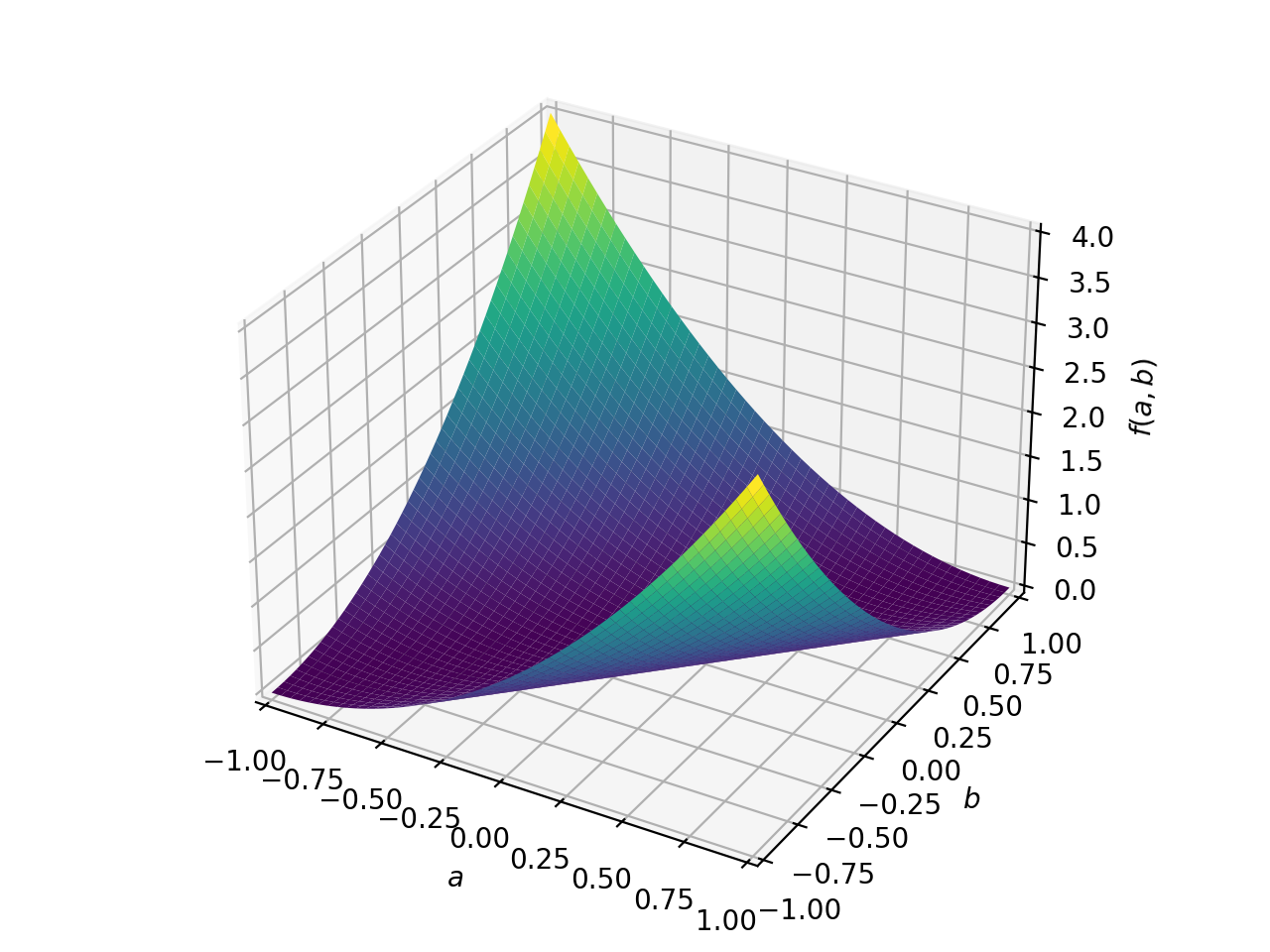
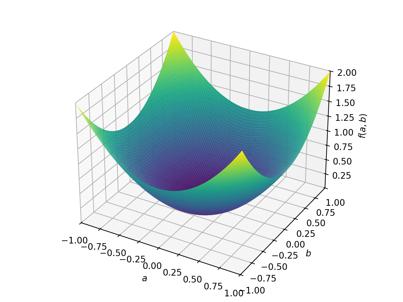
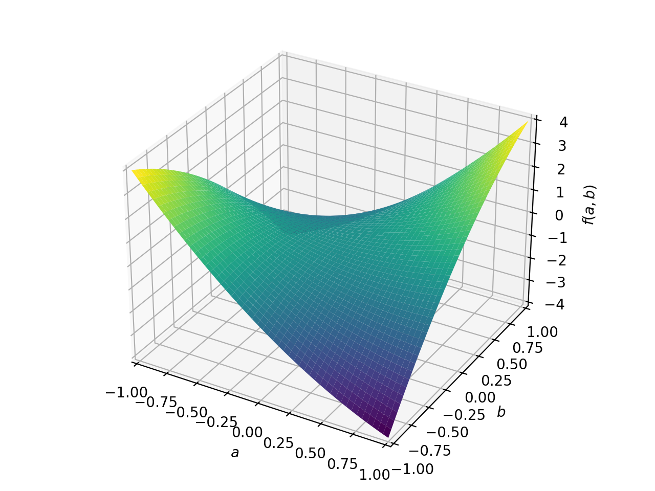
Matrix Exceptions
Matrix Functions
- sympy.matrices.dense.matrix_multiply_elementwise(A, B)[source]
Return the Hadamard product (elementwise product) of A and B
>>> from sympy import Matrix, matrix_multiply_elementwise >>> A = Matrix([[0, 1, 2], [3, 4, 5]]) >>> B = Matrix([[1, 10, 100], [100, 10, 1]]) >>> matrix_multiply_elementwise(A, B) Matrix([ [ 0, 10, 200], [300, 40, 5]])
- sympy.matrices.dense.zeros(*args, **kwargs)[source]
Returns a matrix of zeros with
rowsrows andcolscolumns; ifcolsis omitted a square matrix will be returned.
- sympy.matrices.dense.ones(*args, **kwargs)[source]
Returns a matrix of ones with
rowsrows andcolscolumns; ifcolsis omitted a square matrix will be returned.
- sympy.matrices.dense.diag(*values, strict=True, unpack=False, **kwargs)[source]
Returns a matrix with the provided values placed on the diagonal. If non-square matrices are included, they will produce a block-diagonal matrix.
Examples
This version of diag is a thin wrapper to Matrix.diag that differs in that it treats all lists like matrices – even when a single list is given. If this is not desired, either put a \(*\) before the list or set \(unpack=True\).
>>> from sympy import diag
>>> diag([1, 2, 3], unpack=True) # = diag(1,2,3) or diag(*[1,2,3]) Matrix([ [1, 0, 0], [0, 2, 0], [0, 0, 3]])
>>> diag([1, 2, 3]) # a column vector Matrix([ [1], [2], [3]])
- sympy.matrices.dense.jordan_cell(eigenval, n)[source]
Create a Jordan block:
Examples
>>> from sympy import jordan_cell >>> from sympy.abc import x >>> jordan_cell(x, 4) Matrix([ [x, 1, 0, 0], [0, x, 1, 0], [0, 0, x, 1], [0, 0, 0, x]])
- sympy.matrices.dense.hessian(f, varlist, constraints=())[source]
Compute Hessian matrix for a function f wrt parameters in varlist which may be given as a sequence or a row/column vector. A list of constraints may optionally be given.
Examples
>>> from sympy import Function, hessian, pprint >>> from sympy.abc import x, y >>> f = Function('f')(x, y) >>> g1 = Function('g')(x, y) >>> g2 = x**2 + 3*y >>> pprint(hessian(f, (x, y), [g1, g2])) [ d d ] [ 0 0 --(g(x, y)) --(g(x, y)) ] [ dx dy ] [ ] [ 0 0 2*x 3 ] [ ] [ 2 2 ] [d d d ] [--(g(x, y)) 2*x ---(f(x, y)) -----(f(x, y))] [dx 2 dy dx ] [ dx ] [ ] [ 2 2 ] [d d d ] [--(g(x, y)) 3 -----(f(x, y)) ---(f(x, y)) ] [dy dy dx 2 ] [ dy ]
References
- sympy.matrices.dense.GramSchmidt(vlist, orthonormal=False)[source]
Apply the Gram-Schmidt process to a set of vectors.
- Parameters:
vlist : List of Matrix
Vectors to be orthogonalized for.
orthonormal : Bool, optional
If true, return an orthonormal basis.
- Returns:
vlist : List of Matrix
Orthogonalized vectors
Notes
This routine is mostly duplicate from
Matrix.orthogonalize, except for some difference that this always raises error when linearly dependent vectors are found, and the keywordnormalizehas been named asorthonormalin this function.See also
References
- sympy.matrices.dense.wronskian(functions, var, method='bareiss')[source]
Compute Wronskian for [] of functions
| f1 f2 ... fn | | f1' f2' ... fn' | | . . . . | W(f1, ..., fn) = | . . . . | | . . . . | | (n) (n) (n) | | D (f1) D (f2) ... D (fn) |
- sympy.matrices.dense.casoratian(seqs, n, zero=True)[source]
Given linear difference operator L of order ‘k’ and homogeneous equation Ly = 0 we want to compute kernel of L, which is a set of ‘k’ sequences: a(n), b(n), … z(n).
Solutions of L are linearly independent iff their Casoratian, denoted as C(a, b, …, z), do not vanish for n = 0.
Casoratian is defined by k x k determinant:
+ a(n) b(n) . . . z(n) + | a(n+1) b(n+1) . . . z(n+1) | | . . . . | | . . . . | | . . . . | + a(n+k-1) b(n+k-1) . . . z(n+k-1) +
It proves very useful in rsolve_hyper() where it is applied to a generating set of a recurrence to factor out linearly dependent solutions and return a basis:
>>> from sympy import Symbol, casoratian, factorial >>> n = Symbol('n', integer=True)
Exponential and factorial are linearly independent:
>>> casoratian([2**n, factorial(n)], n) != 0 True
- sympy.matrices.dense.randMatrix(
- r,
- c=None,
- min=0,
- max=99,
- seed=None,
- symmetric=False,
- percent=100,
- prng=None,
Create random matrix with dimensions
rxc. Ifcis omitted the matrix will be square. Ifsymmetricis True the matrix must be square. Ifpercentis less than 100 then only approximately the given percentage of elements will be non-zero.The pseudo-random number generator used to generate matrix is chosen in the following way.
If
prngis supplied, it will be used as random number generator. It should be an instance ofrandom.Random, or at least haverandintandshufflemethods with same signatures.if
prngis not supplied butseedis supplied, then newrandom.Randomwith givenseedwill be created;otherwise, a new
random.Randomwith default seed will be used.
Examples
>>> from sympy import randMatrix >>> randMatrix(3) [25, 45, 27] [44, 54, 9] [23, 96, 46] >>> randMatrix(3, 2) [87, 29] [23, 37] [90, 26] >>> randMatrix(3, 3, 0, 2) [0, 2, 0] [2, 0, 1] [0, 0, 1] >>> randMatrix(3, symmetric=True) [85, 26, 29] [26, 71, 43] [29, 43, 57] >>> A = randMatrix(3, seed=1) >>> B = randMatrix(3, seed=2) >>> A == B False >>> A == randMatrix(3, seed=1) True >>> randMatrix(3, symmetric=True, percent=50) [77, 70, 0], [70, 0, 0], [ 0, 0, 88]
Rotation matrices
- sympy.matrices.dense.rot_givens(i, j, theta, dim=3)[source]
Returns a a Givens rotation matrix, a a rotation in the plane spanned by two coordinates axes.
- Parameters:
i : int between
0anddim - 1Represents first axis
j : int between
0anddim - 1Represents second axis
dim : int bigger than 1
Number of dimensions. Defaults to 3.
Explanation
The Givens rotation corresponds to a generalization of rotation matrices to any number of dimensions, given by:
\[\begin{split}G(i, j, \theta) = \begin{bmatrix} 1 & \cdots & 0 & \cdots & 0 & \cdots & 0 \\ \vdots & \ddots & \vdots & & \vdots & & \vdots \\ 0 & \cdots & c & \cdots & -s & \cdots & 0 \\ \vdots & & \vdots & \ddots & \vdots & & \vdots \\ 0 & \cdots & s & \cdots & c & \cdots & 0 \\ \vdots & & \vdots & & \vdots & \ddots & \vdots \\ 0 & \cdots & 0 & \cdots & 0 & \cdots & 1 \end{bmatrix}\end{split}\]Where \(c = \cos(\theta)\) and \(s = \sin(\theta)\) appear at the intersections
ith andjth rows and columns.For fixed
i > j, the non-zero elements of a Givens matrix are given by:\(g_{kk} = 1\) for \(k \ne i,\,j\)
\(g_{kk} = c\) for \(k = i,\,j\)
\(g_{ji} = -g_{ij} = -s\)
Examples
>>> from sympy import pi, rot_givens
A counterclockwise rotation of pi/3 (60 degrees) around the third axis (z-axis):
>>> rot_givens(1, 0, pi/3) Matrix([ [ 1/2, -sqrt(3)/2, 0], [sqrt(3)/2, 1/2, 0], [ 0, 0, 1]])
If we rotate by pi/2 (90 degrees):
>>> rot_givens(1, 0, pi/2) Matrix([ [0, -1, 0], [1, 0, 0], [0, 0, 1]])
This can be generalized to any number of dimensions:
>>> rot_givens(1, 0, pi/2, dim=4) Matrix([ [0, -1, 0, 0], [1, 0, 0, 0], [0, 0, 1, 0], [0, 0, 0, 1]])
See also
rot_axis1Returns a rotation matrix for a rotation of theta (in radians) about the 1-axis (clockwise around the x axis)
rot_axis2Returns a rotation matrix for a rotation of theta (in radians) about the 2-axis (clockwise around the y axis)
rot_axis3Returns a rotation matrix for a rotation of theta (in radians) about the 3-axis (clockwise around the z axis)
rot_ccw_axis1Returns a rotation matrix for a rotation of theta (in radians) about the 1-axis (counterclockwise around the x axis)
rot_ccw_axis2Returns a rotation matrix for a rotation of theta (in radians) about the 2-axis (counterclockwise around the y axis)
rot_ccw_axis3Returns a rotation matrix for a rotation of theta (in radians) about the 3-axis (counterclockwise around the z axis)
References
- sympy.matrices.dense.rot_axis1(theta)[source]
Returns a rotation matrix for a rotation of theta (in radians) about the 1-axis.
Explanation
For a right-handed coordinate system, this corresponds to a clockwise rotation around the \(x\)-axis, given by:
\[\begin{split}R = \begin{bmatrix} 1 & 0 & 0 \\ 0 & \cos(\theta) & \sin(\theta) \\ 0 & -\sin(\theta) & \cos(\theta) \end{bmatrix}\end{split}\]Examples
>>> from sympy import pi, rot_axis1
A rotation of pi/3 (60 degrees):
>>> theta = pi/3 >>> rot_axis1(theta) Matrix([ [1, 0, 0], [0, 1/2, sqrt(3)/2], [0, -sqrt(3)/2, 1/2]])
If we rotate by pi/2 (90 degrees):
>>> rot_axis1(pi/2) Matrix([ [1, 0, 0], [0, 0, 1], [0, -1, 0]])
See also
rot_givensReturns a Givens rotation matrix (generalized rotation for any number of dimensions)
rot_ccw_axis1Returns a rotation matrix for a rotation of theta (in radians) about the 1-axis (counterclockwise around the x axis)
rot_axis2Returns a rotation matrix for a rotation of theta (in radians) about the 2-axis (clockwise around the y axis)
rot_axis3Returns a rotation matrix for a rotation of theta (in radians) about the 3-axis (clockwise around the z axis)
- sympy.matrices.dense.rot_axis2(theta)[source]
Returns a rotation matrix for a rotation of theta (in radians) about the 2-axis.
Explanation
For a right-handed coordinate system, this corresponds to a clockwise rotation around the \(y\)-axis, given by:
\[\begin{split}R = \begin{bmatrix} \cos(\theta) & 0 & -\sin(\theta) \\ 0 & 1 & 0 \\ \sin(\theta) & 0 & \cos(\theta) \end{bmatrix}\end{split}\]Examples
>>> from sympy import pi, rot_axis2
A rotation of pi/3 (60 degrees):
>>> theta = pi/3 >>> rot_axis2(theta) Matrix([ [ 1/2, 0, -sqrt(3)/2], [ 0, 1, 0], [sqrt(3)/2, 0, 1/2]])
If we rotate by pi/2 (90 degrees):
>>> rot_axis2(pi/2) Matrix([ [0, 0, -1], [0, 1, 0], [1, 0, 0]])
See also
rot_givensReturns a Givens rotation matrix (generalized rotation for any number of dimensions)
rot_ccw_axis2Returns a rotation matrix for a rotation of theta (in radians) about the 2-axis (clockwise around the y axis)
rot_axis1Returns a rotation matrix for a rotation of theta (in radians) about the 1-axis (counterclockwise around the x axis)
rot_axis3Returns a rotation matrix for a rotation of theta (in radians) about the 3-axis (counterclockwise around the z axis)
- sympy.matrices.dense.rot_axis3(theta)[source]
Returns a rotation matrix for a rotation of theta (in radians) about the 3-axis.
Explanation
For a right-handed coordinate system, this corresponds to a clockwise rotation around the \(z\)-axis, given by:
\[\begin{split}R = \begin{bmatrix} \cos(\theta) & \sin(\theta) & 0 \\ -\sin(\theta) & \cos(\theta) & 0 \\ 0 & 0 & 1 \end{bmatrix}\end{split}\]Examples
>>> from sympy import pi, rot_axis3
A rotation of pi/3 (60 degrees):
>>> theta = pi/3 >>> rot_axis3(theta) Matrix([ [ 1/2, sqrt(3)/2, 0], [-sqrt(3)/2, 1/2, 0], [ 0, 0, 1]])
If we rotate by pi/2 (90 degrees):
>>> rot_axis3(pi/2) Matrix([ [ 0, 1, 0], [-1, 0, 0], [ 0, 0, 1]])
See also
rot_givensReturns a Givens rotation matrix (generalized rotation for any number of dimensions)
rot_ccw_axis3Returns a rotation matrix for a rotation of theta (in radians) about the 3-axis (counterclockwise around the z axis)
rot_axis1Returns a rotation matrix for a rotation of theta (in radians) about the 1-axis (clockwise around the x axis)
rot_axis2Returns a rotation matrix for a rotation of theta (in radians) about the 2-axis (clockwise around the y axis)
- sympy.matrices.dense.rot_ccw_axis1(theta)[source]
Returns a rotation matrix for a rotation of theta (in radians) about the 1-axis.
Explanation
For a right-handed coordinate system, this corresponds to a counterclockwise rotation around the \(x\)-axis, given by:
\[\begin{split}R = \begin{bmatrix} 1 & 0 & 0 \\ 0 & \cos(\theta) & -\sin(\theta) \\ 0 & \sin(\theta) & \cos(\theta) \end{bmatrix}\end{split}\]Examples
>>> from sympy import pi, rot_ccw_axis1
A rotation of pi/3 (60 degrees):
>>> theta = pi/3 >>> rot_ccw_axis1(theta) Matrix([ [1, 0, 0], [0, 1/2, -sqrt(3)/2], [0, sqrt(3)/2, 1/2]])
If we rotate by pi/2 (90 degrees):
>>> rot_ccw_axis1(pi/2) Matrix([ [1, 0, 0], [0, 0, -1], [0, 1, 0]])
See also
rot_givensReturns a Givens rotation matrix (generalized rotation for any number of dimensions)
rot_axis1Returns a rotation matrix for a rotation of theta (in radians) about the 1-axis (clockwise around the x axis)
rot_ccw_axis2Returns a rotation matrix for a rotation of theta (in radians) about the 2-axis (counterclockwise around the y axis)
rot_ccw_axis3Returns a rotation matrix for a rotation of theta (in radians) about the 3-axis (counterclockwise around the z axis)
- sympy.matrices.dense.rot_ccw_axis2(theta)[source]
Returns a rotation matrix for a rotation of theta (in radians) about the 2-axis.
Explanation
For a right-handed coordinate system, this corresponds to a counterclockwise rotation around the \(y\)-axis, given by:
\[\begin{split}R = \begin{bmatrix} \cos(\theta) & 0 & \sin(\theta) \\ 0 & 1 & 0 \\ -\sin(\theta) & 0 & \cos(\theta) \end{bmatrix}\end{split}\]Examples
>>> from sympy import pi, rot_ccw_axis2
A rotation of pi/3 (60 degrees):
>>> theta = pi/3 >>> rot_ccw_axis2(theta) Matrix([ [ 1/2, 0, sqrt(3)/2], [ 0, 1, 0], [-sqrt(3)/2, 0, 1/2]])
If we rotate by pi/2 (90 degrees):
>>> rot_ccw_axis2(pi/2) Matrix([ [ 0, 0, 1], [ 0, 1, 0], [-1, 0, 0]])
See also
rot_givensReturns a Givens rotation matrix (generalized rotation for any number of dimensions)
rot_axis2Returns a rotation matrix for a rotation of theta (in radians) about the 2-axis (clockwise around the y axis)
rot_ccw_axis1Returns a rotation matrix for a rotation of theta (in radians) about the 1-axis (counterclockwise around the x axis)
rot_ccw_axis3Returns a rotation matrix for a rotation of theta (in radians) about the 3-axis (counterclockwise around the z axis)
- sympy.matrices.dense.rot_ccw_axis3(theta)[source]
Returns a rotation matrix for a rotation of theta (in radians) about the 3-axis.
Explanation
For a right-handed coordinate system, this corresponds to a counterclockwise rotation around the \(z\)-axis, given by:
\[\begin{split}R = \begin{bmatrix} \cos(\theta) & -\sin(\theta) & 0 \\ \sin(\theta) & \cos(\theta) & 0 \\ 0 & 0 & 1 \end{bmatrix}\end{split}\]Examples
>>> from sympy import pi, rot_ccw_axis3
A rotation of pi/3 (60 degrees):
>>> theta = pi/3 >>> rot_ccw_axis3(theta) Matrix([ [ 1/2, -sqrt(3)/2, 0], [sqrt(3)/2, 1/2, 0], [ 0, 0, 1]])
If we rotate by pi/2 (90 degrees):
>>> rot_ccw_axis3(pi/2) Matrix([ [0, -1, 0], [1, 0, 0], [0, 0, 1]])
See also
rot_givensReturns a Givens rotation matrix (generalized rotation for any number of dimensions)
rot_axis3Returns a rotation matrix for a rotation of theta (in radians) about the 3-axis (clockwise around the z axis)
rot_ccw_axis1Returns a rotation matrix for a rotation of theta (in radians) about the 1-axis (counterclockwise around the x axis)
rot_ccw_axis2Returns a rotation matrix for a rotation of theta (in radians) about the 2-axis (counterclockwise around the y axis)
Numpy Utility Functions
- sympy.matrices.dense.list2numpy(l, dtype=<class 'object'>)[source]
Converts Python list of SymPy expressions to a NumPy array.
See also
- sympy.matrices.dense.matrix2numpy(m, dtype=<class 'object'>)[source]
Converts SymPy’s matrix to a NumPy array.
See also
- sympy.matrices.dense.symarray(prefix, shape, **kwargs)[source]
Create a numpy ndarray of symbols (as an object array).
The created symbols are named
prefix_i1_i2_… You should thus provide a non-empty prefix if you want your symbols to be unique for different output arrays, as SymPy symbols with identical names are the same object.- Parameters:
prefix : string
A prefix prepended to the name of every symbol.
shape : int or tuple
Shape of the created array. If an int, the array is one-dimensional; for more than one dimension the shape must be a tuple.
**kwargs : dict
keyword arguments passed on to Symbol
Examples
These doctests require numpy.
>>> from sympy import symarray >>> symarray('', 3) [_0 _1 _2]
If you want multiple symarrays to contain distinct symbols, you must provide unique prefixes:
>>> a = symarray('', 3) >>> b = symarray('', 3) >>> a[0] == b[0] True >>> a = symarray('a', 3) >>> b = symarray('b', 3) >>> a[0] == b[0] False
Creating symarrays with a prefix:
>>> symarray('a', 3) [a_0 a_1 a_2]
For more than one dimension, the shape must be given as a tuple:
>>> symarray('a', (2, 3)) [[a_0_0 a_0_1 a_0_2] [a_1_0 a_1_1 a_1_2]] >>> symarray('a', (2, 3, 2)) [[[a_0_0_0 a_0_0_1] [a_0_1_0 a_0_1_1] [a_0_2_0 a_0_2_1]] [[a_1_0_0 a_1_0_1] [a_1_1_0 a_1_1_1] [a_1_2_0 a_1_2_1]]]
For setting assumptions of the underlying Symbols:
>>> [s.is_real for s in symarray('a', 2, real=True)] [True, True]