Fourier Series

Provides methods to compute Fourier series.

class sympy.series.fourier.FourierSeries(*args)

Represents Fourier sine/cosine series.

Explanation

This class only represents a fourier series. No computation is performed.

For how to compute Fourier series, see the fourier_series() docstring.

See also

sympy.series.fourier.fourier_series

scale(s)

Scale the function by a term independent of x.

Explanation

f(x) -> s * f(x)

This is fast, if Fourier series of f(x) is already computed.

Examples

>>> from sympy import fourier_series, pi
>>> from sympy.abc import x
>>> s = fourier_series(x**2, (x, -pi, pi))
>>> s.scale(2).truncate()
-8*cos(x) + 2*cos(2*x) + 2*pi**2/3

scalex(s)

Scale x by a term independent of x.

Explanation

f(x) -> f(s*x)

This is fast, if Fourier series of f(x) is already computed.

Examples

>>> from sympy import fourier_series, pi
>>> from sympy.abc import x
>>> s = fourier_series(x**2, (x, -pi, pi))
>>> s.scalex(2).truncate()
-4*cos(2*x) + cos(4*x) + pi**2/3

shift(s)

Shift the function by a term independent of x.

Explanation

f(x) -> f(x) + s

This is fast, if Fourier series of f(x) is already computed.

Examples

>>> from sympy import fourier_series, pi
>>> from sympy.abc import x
>>> s = fourier_series(x**2, (x, -pi, pi))
>>> s.shift(1).truncate()
-4*cos(x) + cos(2*x) + 1 + pi**2/3

shiftx(s)

Shift x by a term independent of x.

Explanation

f(x) -> f(x + s)

This is fast, if Fourier series of f(x) is already computed.

Examples

>>> from sympy import fourier_series, pi
>>> from sympy.abc import x
>>> s = fourier_series(x**2, (x, -pi, pi))
>>> s.shiftx(1).truncate()
-4*cos(x + 1) + cos(2*x + 2) + pi**2/3

sigma_approximation(n=3)

Return \(\sigma\)-approximation of Fourier series with respect to order n.

Parameters:

n : int

Highest order of the terms taken into account in approximation.

Returns:

Expr :

Sigma approximation of function expanded into Fourier series.

Explanation

Sigma approximation adjusts a Fourier summation to eliminate the Gibbs phenomenon which would otherwise occur at discontinuities. A sigma-approximated summation for a Fourier series of a T-periodical function can be written as

\[s(\theta) = \frac{1}{2} a_0 + \sum _{k=1}^{m-1} \operatorname{sinc} \Bigl( \frac{k}{m} \Bigr) \cdot \left[ a_k \cos \Bigl( \frac{2\pi k}{T} \theta \Bigr) + b_k \sin \Bigl( \frac{2\pi k}{T} \theta \Bigr) \right],\]

where \(a_0, a_k, b_k, k=1,\ldots,{m-1}\) are standard Fourier series coefficients and \(\operatorname{sinc} \Bigl( \frac{k}{m} \Bigr)\) is a Lanczos \(\sigma\) factor (expressed in terms of normalized \(\operatorname{sinc}\) function).

Examples

>>> from sympy import fourier_series, pi
>>> from sympy.abc import x
>>> s = fourier_series(x, (x, -pi, pi))
>>> s.sigma_approximation(4)
2*sin(x)*sinc(pi/4) - 2*sin(2*x)/pi + 2*sin(3*x)*sinc(3*pi/4)/3

Notes

The behaviour of sigma_approximation() is different from truncate() - it takes all nonzero terms of degree smaller than n, rather than first n nonzero ones.

See also

sympy.series.fourier.FourierSeries.truncate

References

[R838]

https://en.wikipedia.org/wiki/Gibbs_phenomenon

[R839]

https://en.wikipedia.org/wiki/Sigma_approximation

truncate(n=3)

Return the first n nonzero terms of the series.

If n is None return an iterator.

Parameters:

n : int or None

Amount of non-zero terms in approximation or None.

Returns:

Expr or iterator :

Approximation of function expanded into Fourier series.

Examples

>>> from sympy import fourier_series, pi
>>> from sympy.abc import x
>>> s = fourier_series(x, (x, -pi, pi))
>>> s.truncate(4)
2*sin(x) - sin(2*x) + 2*sin(3*x)/3 - sin(4*x)/2

See also

sympy.series.fourier.FourierSeries.sigma_approximation

sympy.series.fourier.fourier_series(f, limits=None, finite=True)

Computes the Fourier trigonometric series expansion.

Parameters:

limits : (sym, start, end), optional

sym denotes the symbol the series is computed with respect to.

start and end denotes the start and the end of the interval where the fourier series converges to the given function.

Default range is specified as \(-\pi\) and \(\pi\).

Returns:

FourierSeries

A symbolic object representing the Fourier trigonometric series.

Explanation

Fourier trigonometric series of \(f(x)\) over the interval \((a, b)\) is defined as:

\[\frac{a_0}{2} + \sum_{n=1}^{\infty} (a_n \cos(\frac{2n \pi x}{L}) + b_n \sin(\frac{2n \pi x}{L}))\]

where the coefficients are:

\[L = b - a\]

\[a_0 = \frac{2}{L} \int_{a}^{b}{f(x) dx}\]

\[a_n = \frac{2}{L} \int_{a}^{b}{f(x) \cos(\frac{2n \pi x}{L}) dx}\]

\[b_n = \frac{2}{L} \int_{a}^{b}{f(x) \sin(\frac{2n \pi x}{L}) dx}\]

The condition whether the function \(f(x)\) given should be periodic or not is more than necessary, because it is sufficient to consider the series to be converging to \(f(x)\) only in the given interval, not throughout the whole real line.

This also brings a lot of ease for the computation because you do not have to make \(f(x)\) artificially periodic by wrapping it with piecewise, modulo operations, but you can shape the function to look like the desired periodic function only in the interval \((a, b)\), and the computed series will automatically become the series of the periodic version of \(f(x)\).

This property is illustrated in the examples section below.

Examples

Computing the Fourier series of \(f(x) = x^2\):

>>> from sympy import fourier_series, pi
>>> from sympy.abc import x
>>> f = x**2
>>> s = fourier_series(f, (x, -pi, pi))
>>> s1 = s.truncate(n=3)
>>> s1
-4*cos(x) + cos(2*x) + pi**2/3

Shifting of the Fourier series:

>>> s.shift(1).truncate()
-4*cos(x) + cos(2*x) + 1 + pi**2/3
>>> s.shiftx(1).truncate()
-4*cos(x + 1) + cos(2*x + 2) + pi**2/3

Scaling of the Fourier series:

>>> s.scale(2).truncate()
-8*cos(x) + 2*cos(2*x) + 2*pi**2/3
>>> s.scalex(2).truncate()
-4*cos(2*x) + cos(4*x) + pi**2/3

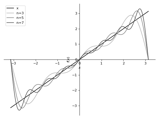
Computing the Fourier series of \(f(x) = x\):

This illustrates how truncating to the higher order gives better convergence.

>>> from sympy import fourier_series, pi, plot
>>> from sympy.abc import x
>>> f = x
>>> s = fourier_series(f, (x, -pi, pi))
>>> s1 = s.truncate(n = 3)
>>> s2 = s.truncate(n = 5)
>>> s3 = s.truncate(n = 7)
>>> p = plot(f, s1, s2, s3, (x, -pi, pi), show=False, legend=True)

>>> p[0].line_color = (0, 0, 0)
>>> p[0].label = 'x'
>>> p[1].line_color = (0.7, 0.7, 0.7)
>>> p[1].label = 'n=3'
>>> p[2].line_color = (0.5, 0.5, 0.5)
>>> p[2].label = 'n=5'
>>> p[3].line_color = (0.3, 0.3, 0.3)
>>> p[3].label = 'n=7'

>>> p.show()

(png, hires.png, pdf)

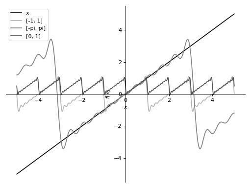
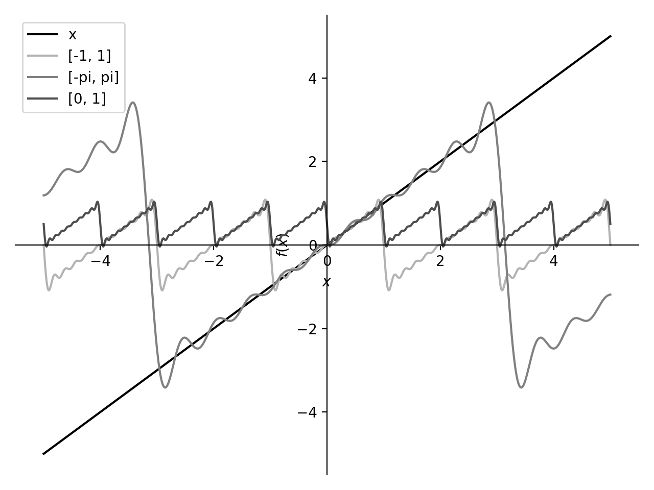
This illustrates how the series converges to different sawtooth waves if the different ranges are specified.

>>> s1 = fourier_series(x, (x, -1, 1)).truncate(10)
>>> s2 = fourier_series(x, (x, -pi, pi)).truncate(10)
>>> s3 = fourier_series(x, (x, 0, 1)).truncate(10)
>>> p = plot(x, s1, s2, s3, (x, -5, 5), show=False, legend=True)

>>> p[0].line_color = (0, 0, 0)
>>> p[0].label = 'x'
>>> p[1].line_color = (0.7, 0.7, 0.7)
>>> p[1].label = '[-1, 1]'
>>> p[2].line_color = (0.5, 0.5, 0.5)
>>> p[2].label = '[-pi, pi]'
>>> p[3].line_color = (0.3, 0.3, 0.3)
>>> p[3].label = '[0, 1]'

>>> p.show()

(png, hires.png, pdf)

Notes

Computing Fourier series can be slow due to the integration required in computing an, bn.

It is faster to compute Fourier series of a function by using shifting and scaling on an already computed Fourier series rather than computing again.

e.g. If the Fourier series of x**2 is known the Fourier series of x**2 - 1 can be found by shifting by -1.

See also

sympy.series.fourier.FourierSeries

References

[R840]

https://mathworld.wolfram.com/FourierSeries.html