Beam (Docstrings)¶

This module can be used to solve 2D beam bending problems with singularity functions in mechanics.

class sympy.physics.continuum_mechanics.beam.Beam( length, elastic_modulus, second_moment, area=A, variable=x, base_char='C', ild_variable=a, )[source]¶

A Beam is a structural element that is capable of withstanding load primarily by resisting against bending. Beams are characterized by their cross sectional profile(Second moment of area), their length and their material.

Note

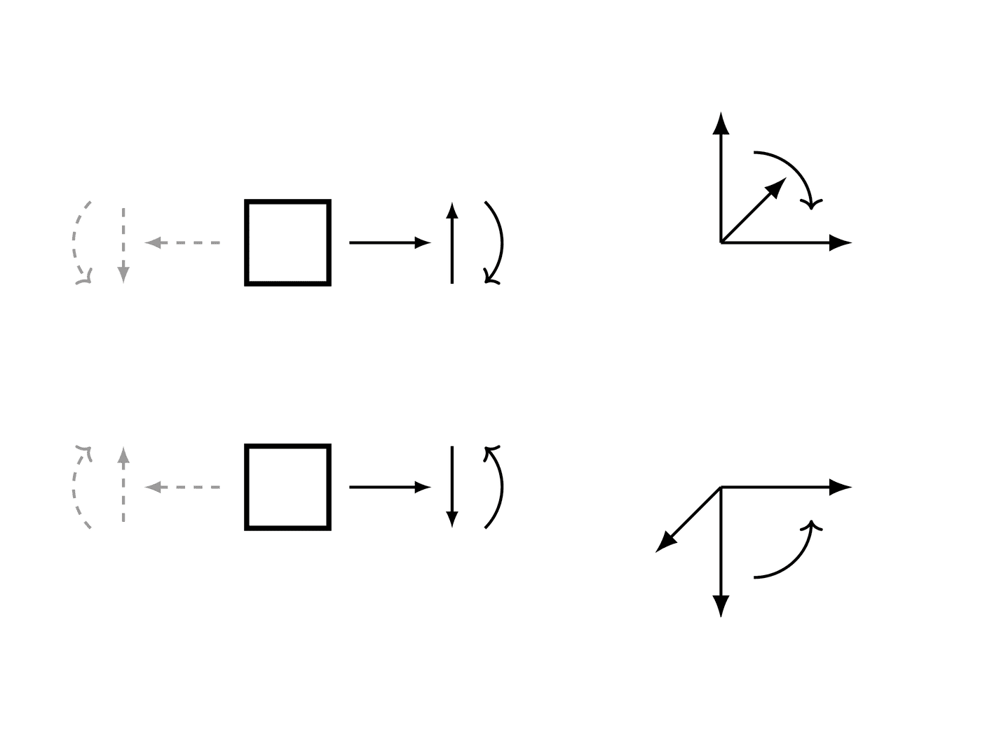
A consistent sign convention must be used while solving a beam bending problem; the results will automatically follow the chosen sign convention. However, the chosen sign convention must respect the rule that, on the positive side of beam’s axis (in respect to current section), a loading force giving positive shear yields a negative moment, as below (the curved arrow shows the positive moment and rotation):

../../../_images/allowed-sign-conventions.png

Examples

There is a beam of length 4 meters. A constant distributed load of 6 N/m is applied from half of the beam till the end. There are two simple supports below the beam, one at the starting point and another at the ending point of the beam. The deflection of the beam at the end is restricted.

Using the sign convention of downwards forces being positive.

>>> from sympy.physics.continuum_mechanics.beam import Beam
>>> from sympy import symbols, Piecewise
>>> E, I = symbols('E, I')
>>> R1, R2 = symbols('R1, R2')
>>> b = Beam(4, E, I)
>>> b.apply_load(R1, 0, -1)
>>> b.apply_load(6, 2, 0)
>>> b.apply_load(R2, 4, -1)
>>> b.bc_deflection = [(0, 0), (4, 0)]
>>> b.boundary_conditions
{'bending_moment': [], 'deflection': [(0, 0), (4, 0)], 'shear_force': [], 'slope': []}
>>> b.load
R1*SingularityFunction(x, 0, -1) + R2*SingularityFunction(x, 4, -1) + 6*SingularityFunction(x, 2, 0)
>>> b.solve_for_reaction_loads(R1, R2)
>>> b.load
-3*SingularityFunction(x, 0, -1) + 6*SingularityFunction(x, 2, 0) - 9*SingularityFunction(x, 4, -1)
>>> b.shear_force()
3*SingularityFunction(x, 0, 0) - 6*SingularityFunction(x, 2, 1) + 9*SingularityFunction(x, 4, 0)
>>> b.bending_moment()
3*SingularityFunction(x, 0, 1) - 3*SingularityFunction(x, 2, 2) + 9*SingularityFunction(x, 4, 1)
>>> b.slope()
(-3*SingularityFunction(x, 0, 2)/2 + SingularityFunction(x, 2, 3) - 9*SingularityFunction(x, 4, 2)/2 + 7)/(E*I)
>>> b.deflection()
(7*x - SingularityFunction(x, 0, 3)/2 + SingularityFunction(x, 2, 4)/4 - 3*SingularityFunction(x, 4, 3)/2)/(E*I)
>>> b.deflection().rewrite(Piecewise)
(7*x - Piecewise((x**3, x >= 0), (0, True))/2
     - 3*Piecewise(((x - 4)**3, x >= 4), (0, True))/2
     + Piecewise(((x - 2)**4, x >= 2), (0, True))/4)/(E*I)

Calculate the support reactions for a fully symbolic beam of length L. There are two simple supports below the beam, one at the starting point and another at the ending point of the beam. The deflection of the beam at the end is restricted. The beam is loaded with:

a downward point load P1 applied at L/4
an upward point load P2 applied at L/8
a counterclockwise moment M1 applied at L/2
a clockwise moment M2 applied at 3*L/4
a distributed constant load q1, applied downward, starting from L/2 up to 3*L/4
a distributed constant load q2, applied upward, starting from 3*L/4 up to L

No assumptions are needed for symbolic loads. However, defining a positive length will help the algorithm to compute the solution.

>>> E, I = symbols('E, I')
>>> L = symbols("L", positive=True)
>>> P1, P2, M1, M2, q1, q2 = symbols("P1, P2, M1, M2, q1, q2")
>>> R1, R2 = symbols('R1, R2')
>>> b = Beam(L, E, I)
>>> b.apply_load(R1, 0, -1)
>>> b.apply_load(R2, L, -1)
>>> b.apply_load(P1, L/4, -1)
>>> b.apply_load(-P2, L/8, -1)
>>> b.apply_load(M1, L/2, -2)
>>> b.apply_load(-M2, 3*L/4, -2)
>>> b.apply_load(q1, L/2, 0, 3*L/4)
>>> b.apply_load(-q2, 3*L/4, 0, L)
>>> b.bc_deflection = [(0, 0), (L, 0)]
>>> b.solve_for_reaction_loads(R1, R2)
>>> print(b.reaction_loads[R1])
(-3*L**2*q1 + L**2*q2 - 24*L*P1 + 28*L*P2 - 32*M1 + 32*M2)/(32*L)
>>> print(b.reaction_loads[R2])
(-5*L**2*q1 + 7*L**2*q2 - 8*L*P1 + 4*L*P2 + 32*M1 - 32*M2)/(32*L)

property applied_loads¶

Returns a list of all loads applied on the beam object. Each load in the list is a tuple of form (value, start, order, end).

Examples

There is a beam of length 4 meters. A moment of magnitude 3 Nm is applied in the clockwise direction at the starting point of the beam. A pointload of magnitude 4 N is applied from the top of the beam at 2 meters from the starting point. Another pointload of magnitude 5 N is applied at same position.

>>> from sympy.physics.continuum_mechanics.beam import Beam
>>> from sympy import symbols
>>> E, I = symbols('E, I')
>>> b = Beam(4, E, I)
>>> b.apply_load(-3, 0, -2)
>>> b.apply_load(4, 2, -1)
>>> b.apply_load(5, 2, -1)
>>> b.load
-3*SingularityFunction(x, 0, -2) + 9*SingularityFunction(x, 2, -1)
>>> b.applied_loads
[(-3, 0, -2, None), (4, 2, -1, None), (5, 2, -1, None)]

apply_load(value, start, order, end=None)[source]¶

This method adds up the loads given to a particular beam object.

Parameters:

value : Sympifyable

The value inserted should have the units [Force/(Distance**(n+1)] where n is the order of applied load. Units for applied loads:

For moments, unit = kN*m

For point loads, unit = kN

For constant distributed load, unit = kN/m

For ramp loads, unit = kN/m/m

For parabolic ramp loads, unit = kN/m/m/m

… so on.

start : Sympifyable

The starting point of the applied load. For point moments and point forces this is the location of application.

order : Integer

The order of the applied load.

For moments, order = -2

For point loads, order =-1

For constant distributed load, order = 0

For ramp loads, order = 1

For parabolic ramp loads, order = 2

… so on.

end : Sympifyable, optional

An optional argument that can be used if the load has an end point within the length of the beam.

Examples

There is a beam of length 4 meters. A moment of magnitude 3 Nm is applied in the clockwise direction at the starting point of the beam. A point load of magnitude 4 N is applied from the top of the beam at 2 meters from the starting point and a parabolic ramp load of magnitude 2 N/m is applied below the beam starting from 2 meters to 3 meters away from the starting point of the beam.

>>> from sympy.physics.continuum_mechanics.beam import Beam
>>> from sympy import symbols
>>> E, I = symbols('E, I')
>>> b = Beam(4, E, I)
>>> b.apply_load(-3, 0, -2)
>>> b.apply_load(4, 2, -1)
>>> b.apply_load(-2, 2, 2, end=3)
>>> b.load
-3*SingularityFunction(x, 0, -2) + 4*SingularityFunction(x, 2, -1) - 2*SingularityFunction(x, 2, 2) + 2*SingularityFunction(x, 3, 0) + 4*SingularityFunction(x, 3, 1) + 2*SingularityFunction(x, 3, 2)

apply_rotation_hinge(loc)[source]¶

This method applies a rotation hinge at a single location on the beam.

Parameters:: loc : Sympifyable

Location of point at which hinge is applied.
Returns:: Symbol

The unknown rotation jump multiplied by the elastic modulus and second moment as a symbol.

Examples

There is a beam of length 15 meters. Pin supports are placed at distances of 0 and 10 meters. There is a fixed support at the end. There are two rotation hinges in the structure, one at 5 meters and one at 10 meters. A pointload of magnitude 10 kN is applied on the hinge at 5 meters. A distributed load of 5 kN works on the structure from 10 meters to the end.

Using the sign convention of upward forces and clockwise moment being positive.

>>> from sympy.physics.continuum_mechanics.beam import Beam
>>> from sympy import Symbol
>>> E = Symbol('E')
>>> I = Symbol('I')
>>> b = Beam(15, E, I)
>>> r0 = b.apply_support(0, type='pin')
>>> r10 = b.apply_support(10, type='pin')
>>> r15, m15 = b.apply_support(15, type='fixed')
>>> p5 = b.apply_rotation_hinge(5)
>>> p12 = b.apply_rotation_hinge(12)
>>> b.apply_load(-10, 5, -1)
>>> b.apply_load(-5, 10, 0, 15)
>>> b.solve_for_reaction_loads(r0, r10, r15, m15)
>>> b.reaction_loads
{M_15: -75/2, R_0: 0, R_10: 40, R_15: -5}
>>> b.rotation_jumps
{P_12: -1875/(16*E*I), P_5: 9625/(24*E*I)}
>>> b.rotation_jumps[p12]
-1875/(16*E*I)
>>> b.bending_moment()
-9625*SingularityFunction(x, 5, -1)/24 + 10*SingularityFunction(x, 5, 1)
- 40*SingularityFunction(x, 10, 1) + 5*SingularityFunction(x, 10, 2)/2
+ 1875*SingularityFunction(x, 12, -1)/16 + 75*SingularityFunction(x, 15, 0)/2
+ 5*SingularityFunction(x, 15, 1) - 5*SingularityFunction(x, 15, 2)/2

apply_sliding_hinge(loc)[source]¶

This method applies a sliding hinge at a single location on the beam.

Parameters:: loc : Sympifyable

Location of point at which hinge is applied.
Returns:: Symbol

The unknown deflection jump multiplied by the elastic modulus and second moment as a symbol.

Examples

There is a beam of length 13 meters. A fixed support is placed at the beginning. There is a pin support at the end. There is a sliding hinge at a location of 8 meters. A pointload of magnitude 10 kN is applied on the hinge at 5 meters.

Using the sign convention of upward forces and clockwise moment being positive.

>>> from sympy.physics.continuum_mechanics.beam import Beam
>>> b = Beam(13, 20, 20)
>>> r0, m0 = b.apply_support(0, type="fixed")
>>> s8 = b.apply_sliding_hinge(8)
>>> r13 = b.apply_support(13, type="pin")
>>> b.apply_load(-10, 5, -1)
>>> b.solve_for_reaction_loads(r0, m0, r13)
>>> b.reaction_loads
{M_0: -50, R_0: 10, R_13: 0}
>>> b.deflection_jumps
{W_8: 85/24}
>>> b.deflection_jumps[s8]
85/24
>>> b.bending_moment()
50*SingularityFunction(x, 0, 0) - 10*SingularityFunction(x, 0, 1)
+ 10*SingularityFunction(x, 5, 1) - 4250*SingularityFunction(x, 8, -2)/3
>>> b.deflection()
-SingularityFunction(x, 0, 2)/16 + SingularityFunction(x, 0, 3)/240
- SingularityFunction(x, 5, 3)/240 + 85*SingularityFunction(x, 8, 0)/24

apply_support(loc, type='fixed')[source]¶

This method applies support to a particular beam object and returns the symbol of the unknown reaction load(s).

Parameters:

loc : Sympifyable

Location of point at which support is applied.

type : String

Determines type of Beam support applied. To apply support structure with - zero degree of freedom, type = “fixed” - one degree of freedom, type = “pin” - two degrees of freedom, type = “roller”

Returns:

Symbol or tuple of Symbol

The unknown reaction load as a symbol. - Symbol(reaction_force) if type = “pin” or “roller” - Symbol(reaction_force), Symbol(reaction_moment) if type = “fixed”

Examples

There is a beam of length 20 meters. A moment of magnitude 100 Nm is applied in the clockwise direction at the end of the beam. A pointload of magnitude 8 N is applied from the top of the beam at a distance of 10 meters. There is one fixed support at the start of the beam and a roller at the end.

Using the sign convention of upward forces and clockwise moment being positive.

>>> from sympy.physics.continuum_mechanics.beam import Beam
>>> from sympy import symbols
>>> E, I = symbols('E, I')
>>> b = Beam(20, E, I)
>>> p0, m0 = b.apply_support(0, 'fixed')
>>> p1 = b.apply_support(20, 'roller')
>>> b.apply_load(-8, 10, -1)
>>> b.apply_load(100, 20, -2)
>>> b.solve_for_reaction_loads(p0, m0, p1)
>>> b.reaction_loads
{M_0: 20, R_0: -2, R_20: 10}
>>> b.reaction_loads[p0]
-2
>>> b.load
20*SingularityFunction(x, 0, -2) - 2*SingularityFunction(x, 0, -1)
- 8*SingularityFunction(x, 10, -1) + 100*SingularityFunction(x, 20, -2)
+ 10*SingularityFunction(x, 20, -1)

property area¶: Cross-sectional area of the Beam.

bending_moment()[source]¶

Returns a Singularity Function expression which represents the bending moment curve of the Beam object.

Examples

There is a beam of length 30 meters. A moment of magnitude 120 Nm is applied in the clockwise direction at the end of the beam. A pointload of magnitude 8 N is applied from the top of the beam at the starting point. There are two simple supports below the beam. One at the end and another one at a distance of 10 meters from the start. The deflection is restricted at both the supports.

Using the sign convention of upward forces and clockwise moment being positive.

>>> from sympy.physics.continuum_mechanics.beam import Beam
>>> from sympy import symbols
>>> E, I = symbols('E, I')
>>> R1, R2 = symbols('R1, R2')
>>> b = Beam(30, E, I)
>>> b.apply_load(-8, 0, -1)
>>> b.apply_load(R1, 10, -1)
>>> b.apply_load(R2, 30, -1)
>>> b.apply_load(120, 30, -2)
>>> b.bc_deflection = [(10, 0), (30, 0)]
>>> b.solve_for_reaction_loads(R1, R2)
>>> b.bending_moment()
8*SingularityFunction(x, 0, 1) - 6*SingularityFunction(x, 10, 1) - 120*SingularityFunction(x, 30, 0) - 2*SingularityFunction(x, 30, 1)

property boundary_conditions¶

Returns a dictionary of boundary conditions applied on the beam. The dictionary has three keywords namely moment, slope and deflection. The value of each keyword is a list of tuple, where each tuple contains location and value of a boundary condition in the format (location, value).

Examples

There is a beam of length 4 meters. The bending moment at 0 should be 4 and at 4 it should be 0. The slope of the beam should be 1 at 0. The deflection should be 2 at 0.

>>> from sympy.physics.continuum_mechanics.beam import Beam
>>> from sympy import symbols
>>> E, I = symbols('E, I')
>>> b = Beam(4, E, I)
>>> b.bc_deflection = [(0, 2)]
>>> b.bc_slope = [(0, 1)]
>>> b.boundary_conditions
{'bending_moment': [], 'deflection': [(0, 2)], 'shear_force': [], 'slope': [(0, 1)]}

Here the deflection of the beam should be 2 at 0. Similarly, the slope of the beam should be 1 at 0.

property cross_section¶: Cross-section of the beam

deflection()[source]¶

Returns a Singularity Function expression which represents the elastic curve or deflection of the Beam object.

Examples

Using the sign convention of upward forces and clockwise moment being positive.

>>> from sympy.physics.continuum_mechanics.beam import Beam
>>> from sympy import symbols
>>> E, I = symbols('E, I')
>>> R1, R2 = symbols('R1, R2')
>>> b = Beam(30, E, I)
>>> b.apply_load(-8, 0, -1)
>>> b.apply_load(R1, 10, -1)
>>> b.apply_load(R2, 30, -1)
>>> b.apply_load(120, 30, -2)
>>> b.bc_deflection = [(10, 0), (30, 0)]
>>> b.solve_for_reaction_loads(R1, R2)
>>> b.deflection()
(4000*x/3 - 4*SingularityFunction(x, 0, 3)/3 + SingularityFunction(x, 10, 3)
    + 60*SingularityFunction(x, 30, 2) + SingularityFunction(x, 30, 3)/3 - 12000)/(E*I)

property deflection_jumps¶: Returns the deflection jumps in sliding hinges in a dictionary. The deflection jump is the deflection (in meters) in a sliding hinge. This can be seen as a jump in the deflection plot.

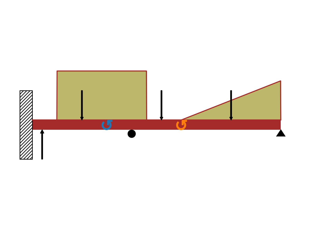
draw(pictorial=True)[source]¶

Returns a plot object representing the beam diagram of the beam. In particular, the diagram might include:

the beam.
vertical black arrows represent point loads and support reaction forces (the latter if they have been added with the apply_load method).
circular arrows represent moments.
shaded areas represent distributed loads.
the support, if apply_support has been executed.
if a composite beam has been created with the join method and a hinge has been specified, it will be shown with a white disc.

The diagram shows positive loads on the upper side of the beam, and negative loads on the lower side. If two or more distributed loads acts along the same direction over the same region, the function will add them up together.

Note

The user must be careful while entering load values. The draw function assumes a sign convention which is used for plotting loads. Given a right handed coordinate system with XYZ coordinates, the beam’s length is assumed to be along the positive X axis. The draw function recognizes positive loads(with n>-2) as loads acting along negative Y direction and positive moments acting along positive Z direction.

Parameters:: pictorial: Boolean (default=True)

Setting pictorial=True would simply create a pictorial (scaled) view of the beam diagram. On the other hand, pictorial=False would create a beam diagram with the exact dimensions on the plot.

Examples

>>> from sympy.physics.continuum_mechanics.beam import Beam
>>> from sympy import symbols
>>> P1, P2, M = symbols('P1, P2, M')
>>> E, I = symbols('E, I')
>>> b = Beam(50, 20, 30)
>>> b.apply_load(-10, 2, -1)
>>> b.apply_load(15, 26, -1)
>>> b.apply_load(P1, 10, -1)
>>> b.apply_load(-P2, 40, -1)
>>> b.apply_load(90, 5, 0, 23)
>>> b.apply_load(10, 30, 1, 50)
>>> b.apply_load(M, 15, -2)
>>> b.apply_load(-M, 30, -2)
>>> p50 = b.apply_support(50, "pin")
>>> p0, m0 = b.apply_support(0, "fixed")
>>> p20 = b.apply_support(20, "roller")
>>> p = b.draw()  
>>> p  
Plot object containing:
[0]: cartesian line: 25*SingularityFunction(x, 5, 0) - 25*SingularityFunction(x, 23, 0)
+ SingularityFunction(x, 30, 1) - 20*SingularityFunction(x, 50, 0)
- SingularityFunction(x, 50, 1) + 5 for x over (0.0, 50.0)
[1]: cartesian line: 5 for x over (0.0, 50.0)
...
>>> p.show() 

(png, hires.png, pdf)

property elastic_modulus¶: Young’s Modulus of the Beam.

property ild_deflection_jumps¶: Returns the I.L.D. deflection jumps in sliding hinges in a dictionary. The deflection jump is the deflection (in meters) in a sliding hinge. This can be seen as a jump in the deflection plot.

property ild_moment¶: Returns the I.L.D. moment equation.

property ild_reactions¶: Returns the I.L.D. reaction forces in a dictionary.

property ild_rotation_jumps¶: Returns the I.L.D. rotation jumps in rotation hinges in a dictionary. The rotation jump is the rotation (in radian) in a rotation hinge. This can be seen as a jump in the slope plot.

property ild_shear¶: Returns the I.L.D. shear equation.

join(beam, via='fixed')[source]¶

This method joins two beams to make a new composite beam system. Passed Beam class instance is attached to the right end of calling object. This method can be used to form beams having Discontinuous values of Elastic modulus or Second moment.

Parameters:

beam : Beam class object

The Beam object which would be connected to the right of calling object.

via : String

States the way two Beam object would get connected - For axially fixed Beams, via=”fixed” - For Beams connected via rotation hinge, via=”hinge”

Examples

There is a cantilever beam of length 4 meters. For first 2 meters its moment of inertia is \(1.5*I\) and \(I\) for the other end. A pointload of magnitude 4 N is applied from the top at its free end.

>>> from sympy.physics.continuum_mechanics.beam import Beam
>>> from sympy import symbols
>>> E, I = symbols('E, I')
>>> R1, R2 = symbols('R1, R2')
>>> b1 = Beam(2, E, 1.5*I)
>>> b2 = Beam(2, E, I)
>>> b = b1.join(b2, "fixed")
>>> b.apply_load(20, 4, -1)
>>> b.apply_load(R1, 0, -1)
>>> b.apply_load(R2, 0, -2)
>>> b.bc_slope = [(0, 0)]
>>> b.bc_deflection = [(0, 0)]
>>> b.solve_for_reaction_loads(R1, R2)
>>> b.load
80*SingularityFunction(x, 0, -2) - 20*SingularityFunction(x, 0, -1) + 20*SingularityFunction(x, 4, -1)
>>> b.slope()
(-((-80*SingularityFunction(x, 0, 1) + 10*SingularityFunction(x, 0, 2) - 10*SingularityFunction(x, 4, 2))/I + 120/I)/E + 80.0/(E*I))*SingularityFunction(x, 2, 0)
- 0.666666666666667*(-80*SingularityFunction(x, 0, 1) + 10*SingularityFunction(x, 0, 2) - 10*SingularityFunction(x, 4, 2))*SingularityFunction(x, 0, 0)/(E*I)
+ 0.666666666666667*(-80*SingularityFunction(x, 0, 1) + 10*SingularityFunction(x, 0, 2) - 10*SingularityFunction(x, 4, 2))*SingularityFunction(x, 2, 0)/(E*I)

property length¶: Length of the Beam.

property load¶

Returns a Singularity Function expression which represents the load distribution curve of the Beam object.

Examples

There is a beam of length 4 meters. A moment of magnitude 3 Nm is applied in the clockwise direction at the starting point of the beam. A point load of magnitude 4 N is applied from the top of the beam at 2 meters from the starting point and a parabolic ramp load of magnitude 2 N/m is applied below the beam starting from 3 meters away from the starting point of the beam.

>>> from sympy.physics.continuum_mechanics.beam import Beam
>>> from sympy import symbols
>>> E, I = symbols('E, I')
>>> b = Beam(4, E, I)
>>> b.apply_load(-3, 0, -2)
>>> b.apply_load(4, 2, -1)
>>> b.apply_load(-2, 3, 2)
>>> b.load
-3*SingularityFunction(x, 0, -2) + 4*SingularityFunction(x, 2, -1) - 2*SingularityFunction(x, 3, 2)

max_bmoment()[source]¶: Returns maximum Shear force and its coordinate in the Beam object.

max_deflection()[source]¶: Returns point of max deflection and its corresponding deflection value in a Beam object.

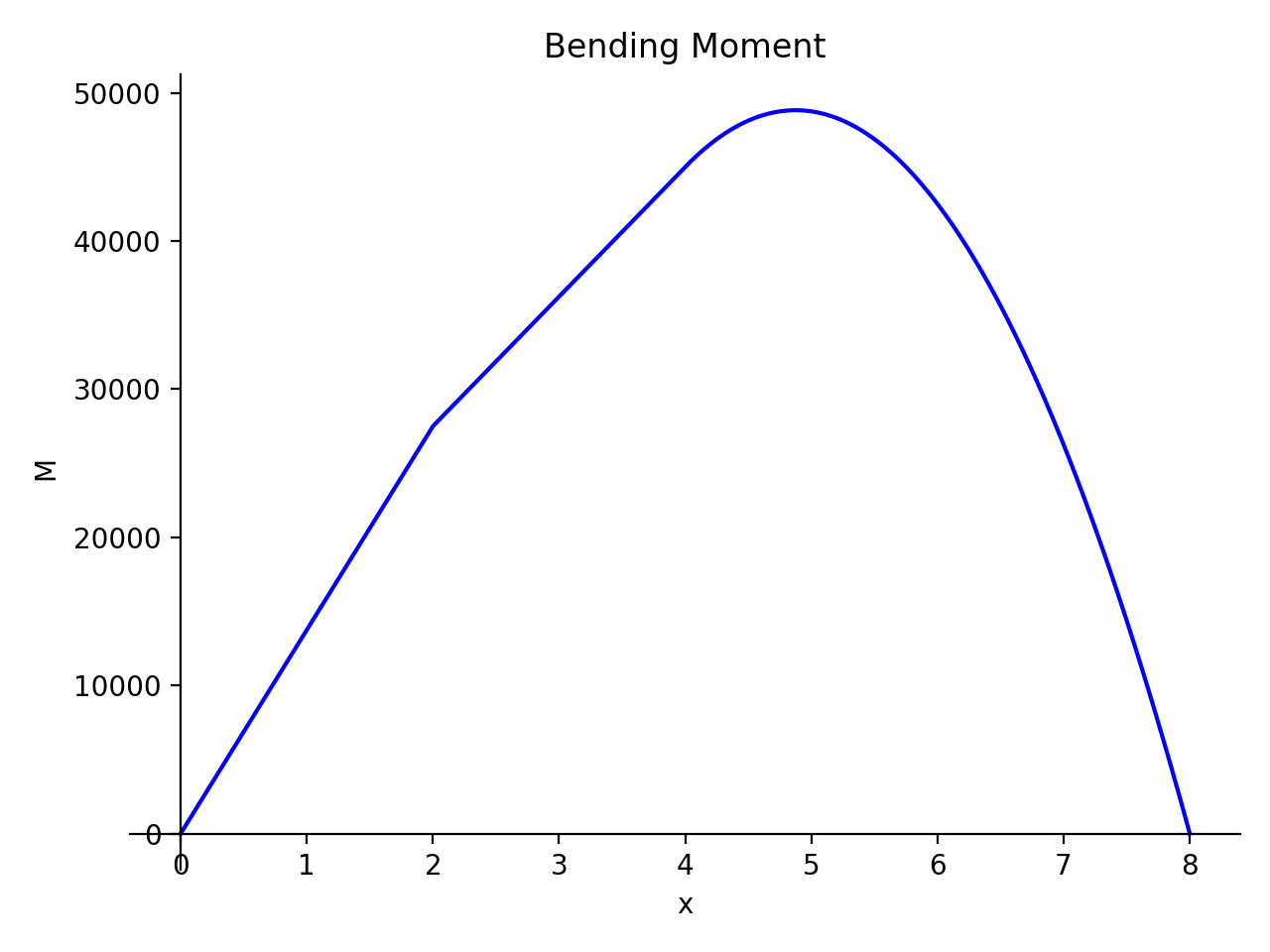
max_shear_force()[source]¶: Returns maximum Shear force and its coordinate in the Beam object.

plot_bending_moment(subs=None)[source]¶

Returns a plot for Bending moment present in the Beam object.

Parameters:: subs : dictionary

Python dictionary containing Symbols as key and their corresponding values.

Examples

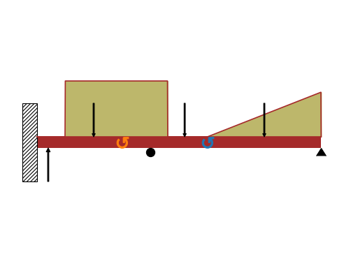
There is a beam of length 8 meters. A constant distributed load of 10 KN/m is applied from half of the beam till the end. There are two simple supports below the beam, one at the starting point and another at the ending point of the beam. A pointload of magnitude 5 KN is also applied from top of the beam, at a distance of 4 meters from the starting point. Take E = 200 GPa and I = 400*(10**-6) meter**4.

Using the sign convention of downwards forces being positive.

>>> from sympy.physics.continuum_mechanics.beam import Beam
>>> from sympy import symbols
>>> R1, R2 = symbols('R1, R2')
>>> b = Beam(8, 200*(10**9), 400*(10**-6))
>>> b.apply_load(5000, 2, -1)
>>> b.apply_load(R1, 0, -1)
>>> b.apply_load(R2, 8, -1)
>>> b.apply_load(10000, 4, 0, end=8)
>>> b.bc_deflection = [(0, 0), (8, 0)]
>>> b.solve_for_reaction_loads(R1, R2)
>>> b.plot_bending_moment()
Plot object containing:
[0]: cartesian line: 13750*SingularityFunction(x, 0, 1) - 5000*SingularityFunction(x, 2, 1)
- 5000*SingularityFunction(x, 4, 2) + 31250*SingularityFunction(x, 8, 1)
+ 5000*SingularityFunction(x, 8, 2) for x over (0.0, 8.0)

(png, hires.png, pdf)

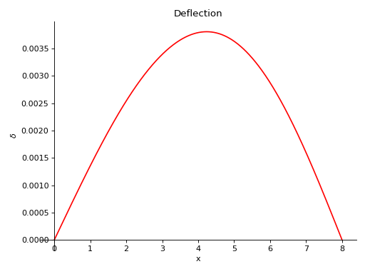
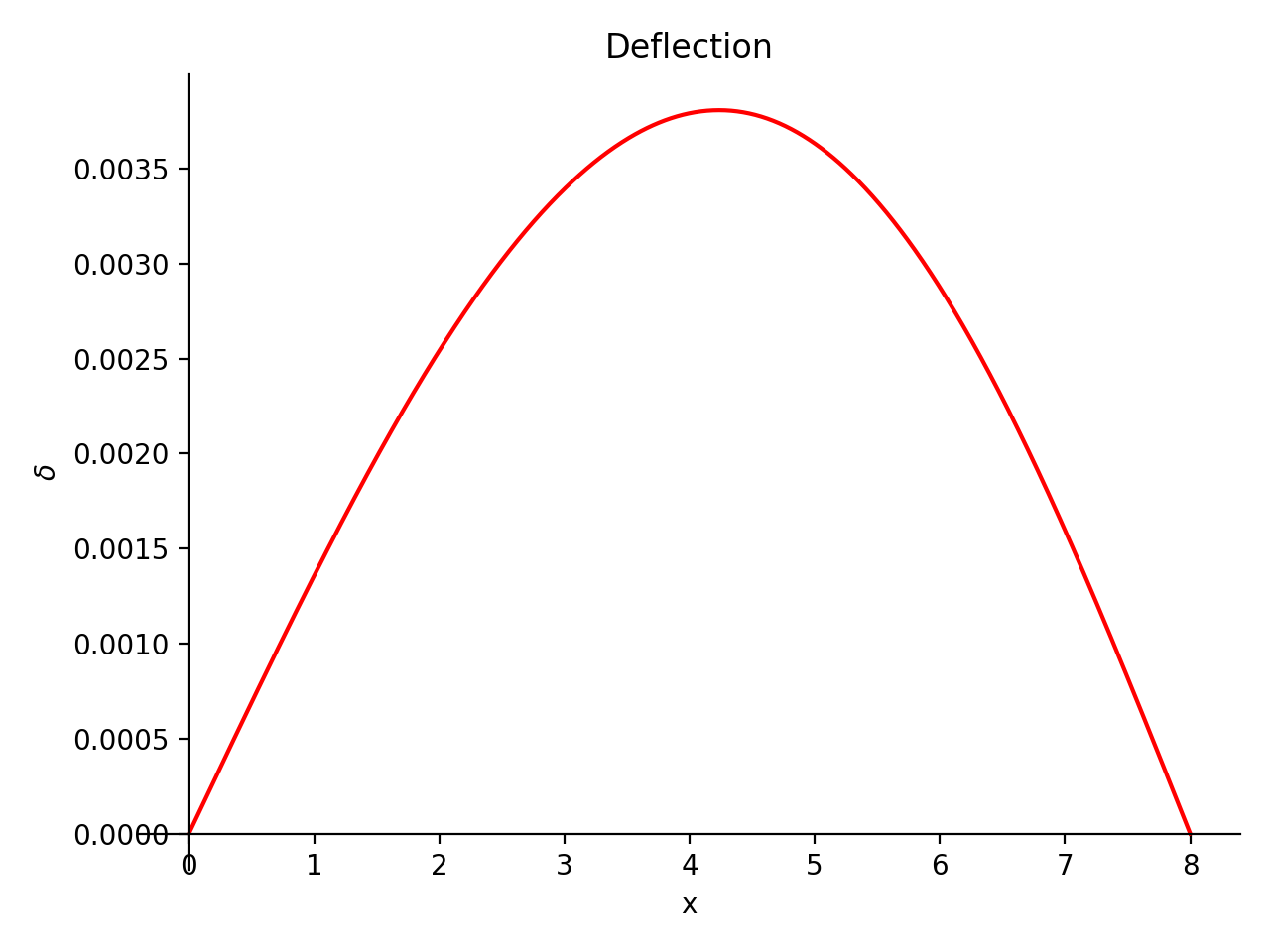
plot_deflection(subs=None)[source]¶

Returns a plot for deflection curve of the Beam object.

Parameters:: subs : dictionary

Python dictionary containing Symbols as key and their corresponding values.

Examples

Using the sign convention of downwards forces being positive.

>>> from sympy.physics.continuum_mechanics.beam import Beam
>>> from sympy import symbols
>>> R1, R2 = symbols('R1, R2')
>>> b = Beam(8, 200*(10**9), 400*(10**-6))
>>> b.apply_load(5000, 2, -1)
>>> b.apply_load(R1, 0, -1)
>>> b.apply_load(R2, 8, -1)
>>> b.apply_load(10000, 4, 0, end=8)
>>> b.bc_deflection = [(0, 0), (8, 0)]
>>> b.solve_for_reaction_loads(R1, R2)
>>> b.plot_deflection()
Plot object containing:
[0]: cartesian line: 0.00138541666666667*x - 2.86458333333333e-5*SingularityFunction(x, 0, 3)
+ 1.04166666666667e-5*SingularityFunction(x, 2, 3) + 5.20833333333333e-6*SingularityFunction(x, 4, 4)
- 6.51041666666667e-5*SingularityFunction(x, 8, 3) - 5.20833333333333e-6*SingularityFunction(x, 8, 4)
for x over (0.0, 8.0)

(png, hires.png, pdf)

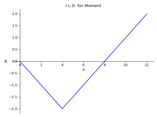
plot_ild_moment(subs=None)[source]¶

Plots the Influence Line Diagram for Moment under the effect of a moving load. This function should be called after calling solve_for_ild_moment().

Parameters:: subs : dictionary

Python dictionary containing Symbols as key and their corresponding values.

Warning

The values for a = 0 and a = l, with l the length of the beam, in the plot can be incorrect.

Examples

There is a beam of length 12 meters. There are two simple supports below the beam, one at the starting point and another at a distance of 8 meters. Plot the I.L.D. for Moment at a distance of 4 meters under the effect of a moving load of magnitude 1kN.

Using the sign convention of downwards forces being positive.

>>> from sympy import symbols
>>> from sympy.physics.continuum_mechanics.beam import Beam
>>> E, I = symbols('E, I')
>>> R_0, R_8 = symbols('R_0, R_8')
>>> b = Beam(12, E, I)
>>> p0 = b.apply_support(0, 'roller')
>>> p8 = b.apply_support(8, 'roller')
>>> b.solve_for_ild_reactions(1, R_0, R_8)
>>> b.solve_for_ild_moment(4, 1, R_0, R_8)
>>> b.ild_moment
-(4*SingularityFunction(a, 0, 0) - SingularityFunction(a, 0, 1) + SingularityFunction(a, 4, 1))*SingularityFunction(a, 4, 0)
- SingularityFunction(a, 0, 1)/2 + SingularityFunction(a, 4, 1) - 2*SingularityFunction(a, 12, 0)
- SingularityFunction(a, 12, 1)/2
>>> b.plot_ild_moment()
Plot object containing:
[0]: cartesian line: -(4*SingularityFunction(a, 0, 0) - SingularityFunction(a, 0, 1)
+ SingularityFunction(a, 4, 1))*SingularityFunction(a, 4, 0) - SingularityFunction(a, 0, 1)/2
+ SingularityFunction(a, 4, 1) - 2*SingularityFunction(a, 12, 0) - SingularityFunction(a, 12, 1)/2 for a over (0.0, 12.0)

(png, hires.png, pdf)

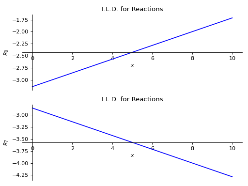
plot_ild_reactions(subs=None)[source]¶

Plots the Influence Line Diagram of Reaction Forces under the effect of a moving load. This function should be called after calling solve_for_ild_reactions().

Parameters:: subs : dictionary

Python dictionary containing Symbols as key and their corresponding values.

Warning

The values for a = 0 and a = l, with l the length of the beam, in the plot can be incorrect.

Examples

There is a beam of length 10 meters. A point load of magnitude 5KN is also applied from top of the beam, at a distance of 4 meters from the starting point. There are two simple supports below the beam, located at the starting point and at a distance of 7 meters from the starting point. Plot the I.L.D. equations for reactions at both support points under the effect of a moving load of magnitude 1kN.

Using the sign convention of downwards forces being positive.

>>> from sympy import symbols
>>> from sympy.physics.continuum_mechanics.beam import Beam
>>> E, I = symbols('E, I')
>>> R_0, R_7 = symbols('R_0, R_7')
>>> b = Beam(10, E, I)
>>> p0 = b.apply_support(0, 'roller')
>>> p7 = b.apply_support(7, 'roller')
>>> b.apply_load(5,4,-1)
>>> b.solve_for_ild_reactions(1,R_0,R_7)
>>> b.ild_reactions
{R_0: -SingularityFunction(a, 0, 0) + SingularityFunction(a, 0, 1)/7
- 3*SingularityFunction(a, 10, 0)/7  - SingularityFunction(a, 10, 1)/7 - 15/7,
R_7: -SingularityFunction(a, 0, 1)/7 + 10*SingularityFunction(a, 10, 0)/7 + SingularityFunction(a, 10, 1)/7 - 20/7}
>>> b.plot_ild_reactions()
PlotGrid object containing:
Plot[0]:Plot object containing:
[0]: cartesian line: -SingularityFunction(a, 0, 0) + SingularityFunction(a, 0, 1)/7
- 3*SingularityFunction(a, 10, 0)/7 - SingularityFunction(a, 10, 1)/7 - 15/7 for a over (0.0, 10.0)
Plot[1]:Plot object containing:
[0]: cartesian line: -SingularityFunction(a, 0, 1)/7 + 10*SingularityFunction(a, 10, 0)/7
+ SingularityFunction(a, 10, 1)/7 - 20/7 for a over (0.0, 10.0)

(png, hires.png, pdf)

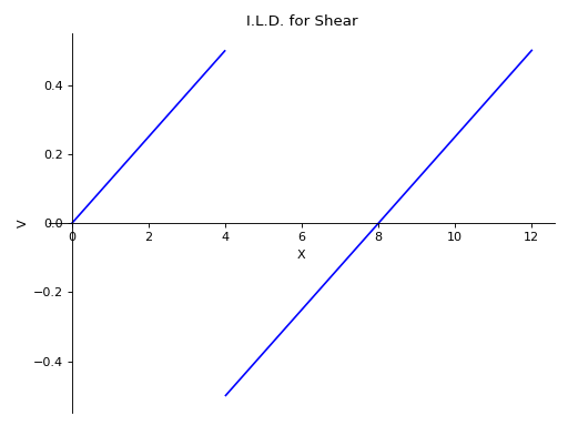
plot_ild_shear(subs=None)[source]¶

Plots the Influence Line Diagram for Shear under the effect of a moving load. This function should be called after calling solve_for_ild_shear().

Parameters:: subs : dictionary

Python dictionary containing Symbols as key and their corresponding values.

Warning

The values for a = 0 and a = l, with l the lenght of the beam, in the plot can be incorrect.

Examples

There is a beam of length 12 meters. There are two simple supports below the beam, one at the starting point and another at a distance of 8 meters. Plot the I.L.D. for Shear at a distance of 4 meters under the effect of a moving load of magnitude 1kN.

Using the sign convention of downwards forces being positive.

>>> from sympy import symbols
>>> from sympy.physics.continuum_mechanics.beam import Beam
>>> E, I = symbols('E, I')
>>> R_0, R_8 = symbols('R_0, R_8')
>>> b = Beam(12, E, I)
>>> p0 = b.apply_support(0, 'roller')
>>> p8 = b.apply_support(8, 'roller')
>>> b.solve_for_ild_reactions(1, R_0, R_8)
>>> b.solve_for_ild_shear(4, 1, R_0, R_8)
>>> b.ild_shear
-(-SingularityFunction(a, 0, 0) + SingularityFunction(a, 12, 0) + 2)*SingularityFunction(a, 4, 0)
- SingularityFunction(-a, 0, 0) - SingularityFunction(a, 0, 0) + SingularityFunction(a, 0, 1)/8
+ SingularityFunction(a, 12, 0)/2 - SingularityFunction(a, 12, 1)/8 + 1
>>> b.plot_ild_shear()
Plot object containing:
[0]: cartesian line: -(-SingularityFunction(a, 0, 0) + SingularityFunction(a, 12, 0) + 2)*SingularityFunction(a, 4, 0)
- SingularityFunction(-a, 0, 0) - SingularityFunction(a, 0, 0) + SingularityFunction(a, 0, 1)/8
+ SingularityFunction(a, 12, 0)/2 - SingularityFunction(a, 12, 1)/8 + 1 for a over (0.0, 12.0)

(png, hires.png, pdf)

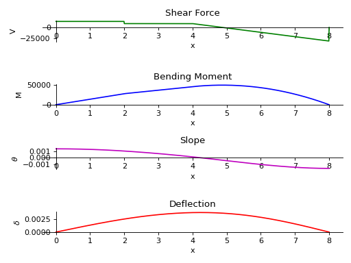
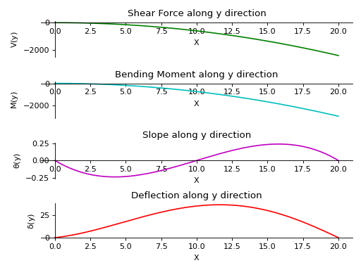
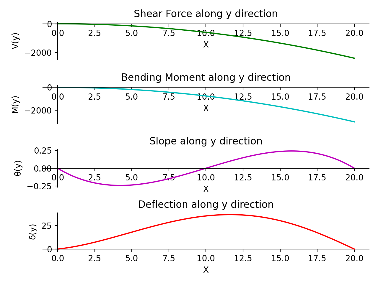
plot_loading_results(subs=None)[source]¶

Returns a subplot of Shear Force, Bending Moment, Slope and Deflection of the Beam object.

Parameters:: subs : dictionary

Python dictionary containing Symbols as key and their corresponding values.

Examples

Using the sign convention of downwards forces being positive.

>>> from sympy.physics.continuum_mechanics.beam import Beam
>>> from sympy import symbols
>>> R1, R2 = symbols('R1, R2')
>>> b = Beam(8, 200*(10**9), 400*(10**-6))
>>> b.apply_load(5000, 2, -1)
>>> b.apply_load(R1, 0, -1)
>>> b.apply_load(R2, 8, -1)
>>> b.apply_load(10000, 4, 0, end=8)
>>> b.bc_deflection = [(0, 0), (8, 0)]
>>> b.solve_for_reaction_loads(R1, R2)
>>> axes = b.plot_loading_results()

(png, hires.png, pdf)

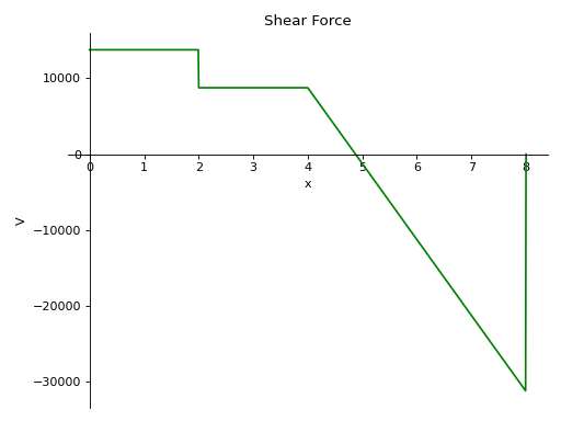
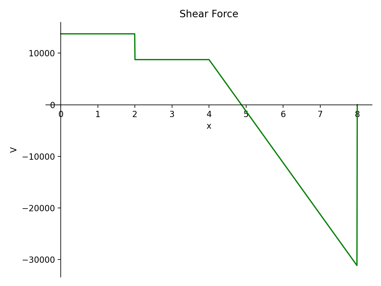
plot_shear_force(subs=None)[source]¶

Returns a plot for Shear force present in the Beam object.

Parameters:: subs : dictionary

Python dictionary containing Symbols as key and their corresponding values.

Examples

Using the sign convention of downwards forces being positive.

>>> from sympy.physics.continuum_mechanics.beam import Beam
>>> from sympy import symbols
>>> R1, R2 = symbols('R1, R2')
>>> b = Beam(8, 200*(10**9), 400*(10**-6))
>>> b.apply_load(5000, 2, -1)
>>> b.apply_load(R1, 0, -1)
>>> b.apply_load(R2, 8, -1)
>>> b.apply_load(10000, 4, 0, end=8)
>>> b.bc_deflection = [(0, 0), (8, 0)]
>>> b.solve_for_reaction_loads(R1, R2)
>>> b.plot_shear_force()
Plot object containing:
[0]: cartesian line: 13750*SingularityFunction(x, 0, 0) - 5000*SingularityFunction(x, 2, 0)
- 10000*SingularityFunction(x, 4, 1) + 31250*SingularityFunction(x, 8, 0)
+ 10000*SingularityFunction(x, 8, 1) for x over (0.0, 8.0)

(png, hires.png, pdf)

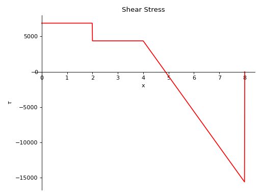
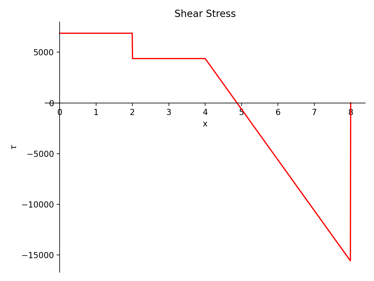
plot_shear_stress(subs=None)[source]¶

Returns a plot of shear stress present in the beam object.

Parameters:: subs : dictionary

Python dictionary containing Symbols as key and their corresponding values.

Examples

There is a beam of length 8 meters and area of cross section 2 square meters. A constant distributed load of 10 KN/m is applied from half of the beam till the end. There are two simple supports below the beam, one at the starting point and another at the ending point of the beam. A pointload of magnitude 5 KN is also applied from top of the beam, at a distance of 4 meters from the starting point. Take E = 200 GPa and I = 400*(10**-6) meter**4.

Using the sign convention of downwards forces being positive.

>>> from sympy.physics.continuum_mechanics.beam import Beam
>>> from sympy import symbols
>>> R1, R2 = symbols('R1, R2')
>>> b = Beam(8, 200*(10**9), 400*(10**-6), 2)
>>> b.apply_load(5000, 2, -1)
>>> b.apply_load(R1, 0, -1)
>>> b.apply_load(R2, 8, -1)
>>> b.apply_load(10000, 4, 0, end=8)
>>> b.bc_deflection = [(0, 0), (8, 0)]
>>> b.solve_for_reaction_loads(R1, R2)
>>> b.plot_shear_stress()
Plot object containing:
[0]: cartesian line: 6875*SingularityFunction(x, 0, 0) - 2500*SingularityFunction(x, 2, 0)
- 5000*SingularityFunction(x, 4, 1) + 15625*SingularityFunction(x, 8, 0)
+ 5000*SingularityFunction(x, 8, 1) for x over (0.0, 8.0)

(png, hires.png, pdf)

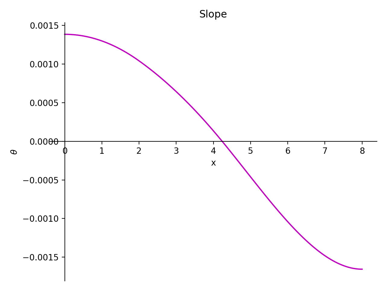
plot_slope(subs=None)[source]¶

Returns a plot for slope of deflection curve of the Beam object.

Parameters:: subs : dictionary

Python dictionary containing Symbols as key and their corresponding values.

Examples

Using the sign convention of downwards forces being positive.

>>> from sympy.physics.continuum_mechanics.beam import Beam
>>> from sympy import symbols
>>> R1, R2 = symbols('R1, R2')
>>> b = Beam(8, 200*(10**9), 400*(10**-6))
>>> b.apply_load(5000, 2, -1)
>>> b.apply_load(R1, 0, -1)
>>> b.apply_load(R2, 8, -1)
>>> b.apply_load(10000, 4, 0, end=8)
>>> b.bc_deflection = [(0, 0), (8, 0)]
>>> b.solve_for_reaction_loads(R1, R2)
>>> b.plot_slope()
Plot object containing:
[0]: cartesian line: -8.59375e-5*SingularityFunction(x, 0, 2) + 3.125e-5*SingularityFunction(x, 2, 2)
+ 2.08333333333333e-5*SingularityFunction(x, 4, 3) - 0.0001953125*SingularityFunction(x, 8, 2)
- 2.08333333333333e-5*SingularityFunction(x, 8, 3) + 0.00138541666666667 for x over (0.0, 8.0)

(png, hires.png, pdf)

point_cflexure()[source]¶

Returns a Set of point(s) with zero bending moment and where bending moment curve of the beam object changes its sign from negative to positive or vice versa.

Examples

There is is 10 meter long overhanging beam. There are two simple supports below the beam. One at the start and another one at a distance of 6 meters from the start. Point loads of magnitude 10KN and 20KN are applied at 2 meters and 4 meters from start respectively. A Uniformly distribute load of magnitude of magnitude 3KN/m is also applied on top starting from 6 meters away from starting point till end. Using the sign convention of upward forces and clockwise moment being positive.

>>> from sympy.physics.continuum_mechanics.beam import Beam
>>> from sympy import symbols
>>> E, I = symbols('E, I')
>>> b = Beam(10, E, I)
>>> b.apply_load(-4, 0, -1)
>>> b.apply_load(-46, 6, -1)
>>> b.apply_load(10, 2, -1)
>>> b.apply_load(20, 4, -1)
>>> b.apply_load(3, 6, 0)
>>> b.point_cflexure()
[10/3]

property reaction_loads¶: Returns the reaction forces in a dictionary.

remove_load(value, start, order, end=None)[source]¶

This method removes a particular load present on the beam object. Returns a ValueError if the load passed as an argument is not present on the beam.

Parameters:

value : Sympifyable

The magnitude of an applied load.

start : Sympifyable

The starting point of the applied load. For point moments and point forces this is the location of application.

order : Integer

The order of the applied load. - For moments, order= -2 - For point loads, order=-1 - For constant distributed load, order=0 - For ramp loads, order=1 - For parabolic ramp loads, order=2 - … so on.

end : Sympifyable, optional

An optional argument that can be used if the load has an end point within the length of the beam.

Examples

There is a beam of length 4 meters. A moment of magnitude 3 Nm is applied in the clockwise direction at the starting point of the beam. A pointload of magnitude 4 N is applied from the top of the beam at 2 meters from the starting point and a parabolic ramp load of magnitude 2 N/m is applied below the beam starting from 2 meters to 3 meters away from the starting point of the beam.

>>> from sympy.physics.continuum_mechanics.beam import Beam
>>> from sympy import symbols
>>> E, I = symbols('E, I')
>>> b = Beam(4, E, I)
>>> b.apply_load(-3, 0, -2)
>>> b.apply_load(4, 2, -1)
>>> b.apply_load(-2, 2, 2, end=3)
>>> b.load
-3*SingularityFunction(x, 0, -2) + 4*SingularityFunction(x, 2, -1) - 2*SingularityFunction(x, 2, 2) + 2*SingularityFunction(x, 3, 0) + 4*SingularityFunction(x, 3, 1) + 2*SingularityFunction(x, 3, 2)
>>> b.remove_load(-2, 2, 2, end = 3)
>>> b.load
-3*SingularityFunction(x, 0, -2) + 4*SingularityFunction(x, 2, -1)

property rotation_jumps¶: Returns the value for the rotation jumps in rotation hinges in a dictionary. The rotation jump is the rotation (in radian) in a rotation hinge. This can be seen as a jump in the slope plot.

property second_moment¶: Second moment of area of the Beam.

shear_force()[source]¶

Returns a Singularity Function expression which represents the shear force curve of the Beam object.

Examples

Using the sign convention of upward forces and clockwise moment being positive.

>>> from sympy.physics.continuum_mechanics.beam import Beam
>>> from sympy import symbols
>>> E, I = symbols('E, I')
>>> R1, R2 = symbols('R1, R2')
>>> b = Beam(30, E, I)
>>> b.apply_load(-8, 0, -1)
>>> b.apply_load(R1, 10, -1)
>>> b.apply_load(R2, 30, -1)
>>> b.apply_load(120, 30, -2)
>>> b.bc_deflection = [(10, 0), (30, 0)]
>>> b.solve_for_reaction_loads(R1, R2)
>>> b.shear_force()
8*SingularityFunction(x, 0, 0) - 6*SingularityFunction(x, 10, 0) - 120*SingularityFunction(x, 30, -1) - 2*SingularityFunction(x, 30, 0)

shear_stress()[source]¶: Returns an expression representing the Shear Stress curve of the Beam object.

slope()[source]¶

Returns a Singularity Function expression which represents the slope the elastic curve of the Beam object.

Examples

Using the sign convention of upward forces and clockwise moment being positive.

>>> from sympy.physics.continuum_mechanics.beam import Beam
>>> from sympy import symbols
>>> E, I = symbols('E, I')
>>> R1, R2 = symbols('R1, R2')
>>> b = Beam(30, E, I)
>>> b.apply_load(-8, 0, -1)
>>> b.apply_load(R1, 10, -1)
>>> b.apply_load(R2, 30, -1)
>>> b.apply_load(120, 30, -2)
>>> b.bc_deflection = [(10, 0), (30, 0)]
>>> b.solve_for_reaction_loads(R1, R2)
>>> b.slope()
(-4*SingularityFunction(x, 0, 2) + 3*SingularityFunction(x, 10, 2)
    + 120*SingularityFunction(x, 30, 1) + SingularityFunction(x, 30, 2) + 4000/3)/(E*I)

solve_for_ild_moment( distance, value, *reactions, )[source]¶

Determines the Influence Line Diagram equations for moment at a specified point under the effect of a moving load.

Parameters:

distance : Integer

Distance of the point from the start of the beam for which equations are to be determined

value : Integer

Magnitude of moving load

reactions :

The reaction forces applied on the beam.

Warning

This method creates equations that can give incorrect results when substituting a = 0 or a = l, with l the lenght of the beam.

Examples

There is a beam of length 12 meters. There are two simple supports below the beam, one at the starting point and another at a distance of 8 meters. Calculate the I.L.D. equations for Moment at a distance of 4 meters under the effect of a moving load of magnitude 1kN.

Using the sign convention of downwards forces being positive.

>>> from sympy import symbols
>>> from sympy.physics.continuum_mechanics.beam import Beam
>>> E, I = symbols('E, I')
>>> R_0, R_8 = symbols('R_0, R_8')
>>> b = Beam(12, E, I)
>>> p0 = b.apply_support(0, 'roller')
>>> p8 = b.apply_support(8, 'roller')
>>> b.solve_for_ild_reactions(1, R_0, R_8)
>>> b.solve_for_ild_moment(4, 1, R_0, R_8)
>>> b.ild_moment
-(4*SingularityFunction(a, 0, 0) - SingularityFunction(a, 0, 1) + SingularityFunction(a, 4, 1))*SingularityFunction(a, 4, 0)
- SingularityFunction(a, 0, 1)/2 + SingularityFunction(a, 4, 1) - 2*SingularityFunction(a, 12, 0)
- SingularityFunction(a, 12, 1)/2

solve_for_ild_reactions(value, *reactions)[source]¶

Determines the Influence Line Diagram equations for reaction forces under the effect of a moving load.

Parameters:

value : Integer

Magnitude of moving load

reactions :

The reaction forces applied on the beam.

Warning

This method creates equations that can give incorrect results when substituting a = 0 or a = l, with l the length of the beam.

Examples

There is a beam of length 10 meters. There are two simple supports below the beam, one at the starting point and another at the ending point of the beam. Calculate the I.L.D. equations for reaction forces under the effect of a moving load of magnitude 1kN.

Using the sign convention of downwards forces being positive.

>>> from sympy import symbols
>>> from sympy.physics.continuum_mechanics.beam import Beam
>>> E, I = symbols('E, I')
>>> R_0, R_10 = symbols('R_0, R_10')
>>> b = Beam(10, E, I)
>>> p0 = b.apply_support(0, 'pin')
>>> p10 = b.apply_support(10, 'roller')
>>> b.solve_for_ild_reactions(1,R_0,R_10)
>>> b.ild_reactions
{R_0: -SingularityFunction(a, 0, 0) + SingularityFunction(a, 0, 1)/10 - SingularityFunction(a, 10, 1)/10,
R_10: -SingularityFunction(a, 0, 1)/10 + SingularityFunction(a, 10, 0) + SingularityFunction(a, 10, 1)/10}

solve_for_ild_shear( distance, value, *reactions, )[source]¶

Determines the Influence Line Diagram equations for shear at a specified point under the effect of a moving load.

Parameters:

distance : Integer

Distance of the point from the start of the beam for which equations are to be determined

value : Integer

Magnitude of moving load

reactions :

The reaction forces applied on the beam.

Warning

This method creates equations that can give incorrect results when substituting a = 0 or a = l, with l the length of the beam.

Examples

There is a beam of length 12 meters. There are two simple supports below the beam, one at the starting point and another at a distance of 8 meters. Calculate the I.L.D. equations for Shear at a distance of 4 meters under the effect of a moving load of magnitude 1kN.

Using the sign convention of downwards forces being positive.

>>> from sympy import symbols
>>> from sympy.physics.continuum_mechanics.beam import Beam
>>> E, I = symbols('E, I')
>>> R_0, R_8 = symbols('R_0, R_8')
>>> b = Beam(12, E, I)
>>> p0 = b.apply_support(0, 'roller')
>>> p8 = b.apply_support(8, 'roller')
>>> b.solve_for_ild_reactions(1, R_0, R_8)
>>> b.solve_for_ild_shear(4, 1, R_0, R_8)
>>> b.ild_shear
-(-SingularityFunction(a, 0, 0) + SingularityFunction(a, 12, 0) + 2)*SingularityFunction(a, 4, 0)
- SingularityFunction(-a, 0, 0) - SingularityFunction(a, 0, 0) + SingularityFunction(a, 0, 1)/8
+ SingularityFunction(a, 12, 0)/2 - SingularityFunction(a, 12, 1)/8 + 1

solve_for_reaction_loads(*reactions)[source]¶

Solves for the reaction forces.

Examples

Using the sign convention of upward forces and clockwise moment being positive.

>>> from sympy.physics.continuum_mechanics.beam import Beam
>>> from sympy import symbols
>>> E, I = symbols('E, I')
>>> R1, R2 = symbols('R1, R2')
>>> b = Beam(30, E, I)
>>> b.apply_load(-8, 0, -1)
>>> b.apply_load(R1, 10, -1)  # Reaction force at x = 10
>>> b.apply_load(R2, 30, -1)  # Reaction force at x = 30
>>> b.apply_load(120, 30, -2)
>>> b.bc_deflection = [(10, 0), (30, 0)]
>>> b.load
R1*SingularityFunction(x, 10, -1) + R2*SingularityFunction(x, 30, -1)
    - 8*SingularityFunction(x, 0, -1) + 120*SingularityFunction(x, 30, -2)
>>> b.solve_for_reaction_loads(R1, R2)
>>> b.reaction_loads
{R1: 6, R2: 2}
>>> b.load
-8*SingularityFunction(x, 0, -1) + 6*SingularityFunction(x, 10, -1)
    + 120*SingularityFunction(x, 30, -2) + 2*SingularityFunction(x, 30, -1)

property variable¶

A symbol that can be used as a variable along the length of the beam while representing load distribution, shear force curve, bending moment, slope curve and the deflection curve. By default, it is set to Symbol('x'), but this property is mutable.

Examples

>>> from sympy.physics.continuum_mechanics.beam import Beam
>>> from sympy import symbols
>>> E, I, A = symbols('E, I, A')
>>> x, y, z = symbols('x, y, z')
>>> b = Beam(4, E, I)
>>> b.variable
x
>>> b.variable = y
>>> b.variable
y
>>> b = Beam(4, E, I, A, z)
>>> b.variable
z

class sympy.physics.continuum_mechanics.beam.Beam3D( length, elastic_modulus, shear_modulus, second_moment, area, variable=x, )[source]¶

This class handles loads applied in any direction of a 3D space along with unequal values of Second moment along different axes.

Note

A consistent sign convention must be used while solving a beam bending problem; the results will automatically follow the chosen sign convention. This class assumes that any kind of distributed load/moment is applied through out the span of a beam.

Examples

There is a beam of l meters long. A constant distributed load of magnitude q is applied along y-axis from start till the end of beam. A constant distributed moment of magnitude m is also applied along z-axis from start till the end of beam. Beam is fixed at both of its end. So, deflection of the beam at the both ends is restricted.

>>> from sympy.physics.continuum_mechanics.beam import Beam3D
>>> from sympy import symbols, simplify, collect, factor
>>> l, E, G, I, A = symbols('l, E, G, I, A')
>>> b = Beam3D(l, E, G, I, A)
>>> x, q, m = symbols('x, q, m')
>>> b.apply_load(q, 0, 0, dir="y")
>>> b.apply_moment_load(m, 0, -1, dir="z")
>>> b.shear_force()
[0, -q*x, 0]
>>> b.bending_moment()
[0, 0, -m*x + q*x**2/2]
>>> b.bc_slope = [(0, [0, 0, 0]), (l, [0, 0, 0])]
>>> b.bc_deflection = [(0, [0, 0, 0]), (l, [0, 0, 0])]
>>> b.solve_slope_deflection()
>>> factor(b.slope())
[0, 0, x*(-l + x)*(-A*G*l**3*q + 2*A*G*l**2*q*x - 12*E*I*l*q
    - 72*E*I*m + 24*E*I*q*x)/(12*E*I*(A*G*l**2 + 12*E*I))]
>>> dx, dy, dz = b.deflection()
>>> dy = collect(simplify(dy), x)
>>> dx == dz == 0
True
>>> dy == (x*(12*E*I*l*(A*G*l**2*q - 2*A*G*l*m + 12*E*I*q)
... + x*(A*G*l*(3*l*(A*G*l**2*q - 2*A*G*l*m + 12*E*I*q) + x*(-2*A*G*l**2*q + 4*A*G*l*m - 24*E*I*q))
... + A*G*(A*G*l**2 + 12*E*I)*(-2*l**2*q + 6*l*m - 4*m*x + q*x**2)
... - 12*E*I*q*(A*G*l**2 + 12*E*I)))/(24*A*E*G*I*(A*G*l**2 + 12*E*I)))
True

References

[R729]

https://homes.civil.aau.dk/jc/FemteSemester/Beams3D.pdf

angular_deflection()[source]¶: Returns a function in x depicting how the angular deflection, due to moments in the x-axis on the beam, varies with x.

apply_load(value, start, order, dir='y')[source]¶

This method adds up the force load to a particular beam object.

Parameters:

value : Sympifyable

The magnitude of an applied load.

dir : String

Axis along which load is applied.

order : Integer

The order of the applied load. - For point loads, order=-1 - For constant distributed load, order=0 - For ramp loads, order=1 - For parabolic ramp loads, order=2 - … so on.

apply_moment_load( value, start, order, dir='y', )[source]¶

This method adds up the moment loads to a particular beam object.

Parameters:

value : Sympifyable

The magnitude of an applied moment.

dir : String

Axis along which moment is applied.

order : Integer

The order of the applied load. - For point moments, order=-2 - For constant distributed moment, order=-1 - For ramp moments, order=0 - For parabolic ramp moments, order=1 - … so on.

property area¶: Cross-sectional area of the Beam.

axial_force()[source]¶: Returns expression of Axial shear force present inside the Beam object.

axial_stress()[source]¶: Returns expression of Axial stress present inside the Beam object.

bending_moment()[source]¶: Returns a list of three expressions which represents the bending moment curve of the Beam object along all three axes.

property boundary_conditions¶

Returns a dictionary of boundary conditions applied on the beam. The dictionary has two keywords namely slope and deflection. The value of each keyword is a list of tuple, where each tuple contains location and value of a boundary condition in the format (location, value). Further each value is a list corresponding to slope or deflection(s) values along three axes at that location.

Examples

There is a beam of length 4 meters. The slope at 0 should be 4 along the x-axis and 0 along others. At the other end of beam, deflection along all the three axes should be zero.

>>> from sympy.physics.continuum_mechanics.beam import Beam3D
>>> from sympy import symbols
>>> l, E, G, I, A, x = symbols('l, E, G, I, A, x')
>>> b = Beam3D(30, E, G, I, A, x)
>>> b.bc_slope = [(0, (4, 0, 0))]
>>> b.bc_deflection = [(4, [0, 0, 0])]
>>> b.boundary_conditions
{'bending_moment': [], 'deflection': [(4, [0, 0, 0])], 'shear_force': [], 'slope': [(0, (4, 0, 0))]}

Here the deflection of the beam should be 0 along all the three axes at 4. Similarly, the slope of the beam should be 4 along x-axis and 0 along y and z axis at 0.

deflection()[source]¶: Returns a three element list representing deflection curve along all the three axes.

property load_vector¶: Returns a three element list representing the load vector.

max_bending_moment()[source]¶

Returns point of max bending moment and its corresponding bending moment value along all directions in a Beam object as a list. solve_for_reaction_loads() must be called before using this function.

Examples

There is a beam of length 20 meters. It is supported by rollers at both of its ends. A linear load having slope equal to 12 is applied along y-axis. A constant distributed load of magnitude 15 N is applied from start till its end along z-axis.

>>> from sympy.physics.continuum_mechanics.beam import Beam3D
>>> from sympy import symbols
>>> l, E, G, I, A, x = symbols('l, E, G, I, A, x')
>>> b = Beam3D(20, 40, 21, 100, 25, x)
>>> b.apply_load(15, start=0, order=0, dir="z")
>>> b.apply_load(12*x, start=0, order=0, dir="y")
>>> b.bc_deflection = [(0, [0, 0, 0]), (20, [0, 0, 0])]
>>> R1, R2, R3, R4 = symbols('R1, R2, R3, R4')
>>> b.apply_load(R1, start=0, order=-1, dir="z")
>>> b.apply_load(R2, start=20, order=-1, dir="z")
>>> b.apply_load(R3, start=0, order=-1, dir="y")
>>> b.apply_load(R4, start=20, order=-1, dir="y")
>>> b.solve_for_reaction_loads(R1, R2, R3, R4)
>>> b.max_bending_moment()
[(0, 0), (20, 3000), (20, 16000)]

max_bmoment()[source]¶

Returns point of max bending moment and its corresponding bending moment value along all directions in a Beam object as a list. solve_for_reaction_loads() must be called before using this function.

Examples

>>> from sympy.physics.continuum_mechanics.beam import Beam3D
>>> from sympy import symbols
>>> l, E, G, I, A, x = symbols('l, E, G, I, A, x')
>>> b = Beam3D(20, 40, 21, 100, 25, x)
>>> b.apply_load(15, start=0, order=0, dir="z")
>>> b.apply_load(12*x, start=0, order=0, dir="y")
>>> b.bc_deflection = [(0, [0, 0, 0]), (20, [0, 0, 0])]
>>> R1, R2, R3, R4 = symbols('R1, R2, R3, R4')
>>> b.apply_load(R1, start=0, order=-1, dir="z")
>>> b.apply_load(R2, start=20, order=-1, dir="z")
>>> b.apply_load(R3, start=0, order=-1, dir="y")
>>> b.apply_load(R4, start=20, order=-1, dir="y")
>>> b.solve_for_reaction_loads(R1, R2, R3, R4)
>>> b.max_bending_moment()
[(0, 0), (20, 3000), (20, 16000)]

max_deflection()[source]¶

Returns point of max deflection and its corresponding deflection value along all directions in a Beam object as a list. solve_for_reaction_loads() and solve_slope_deflection() must be called before using this function.

Examples

>>> from sympy.physics.continuum_mechanics.beam import Beam3D
>>> from sympy import symbols
>>> l, E, G, I, A, x = symbols('l, E, G, I, A, x')
>>> b = Beam3D(20, 40, 21, 100, 25, x)
>>> b.apply_load(15, start=0, order=0, dir="z")
>>> b.apply_load(12*x, start=0, order=0, dir="y")
>>> b.bc_deflection = [(0, [0, 0, 0]), (20, [0, 0, 0])]
>>> R1, R2, R3, R4 = symbols('R1, R2, R3, R4')
>>> b.apply_load(R1, start=0, order=-1, dir="z")
>>> b.apply_load(R2, start=20, order=-1, dir="z")
>>> b.apply_load(R3, start=0, order=-1, dir="y")
>>> b.apply_load(R4, start=20, order=-1, dir="y")
>>> b.solve_for_reaction_loads(R1, R2, R3, R4)
>>> b.solve_slope_deflection()
>>> b.max_deflection()
[(0, 0), (10, 495/14), (-10 + 10*sqrt(10793)/43, (10 - 10*sqrt(10793)/43)**3/160 - 20/7 + (10 - 10*sqrt(10793)/43)**4/6400 + 20*sqrt(10793)/301 + 27*(10 - 10*sqrt(10793)/43)**2/560)]

max_shear_force()[source]¶

Returns point of max shear force and its corresponding shear value along all directions in a Beam object as a list. solve_for_reaction_loads() must be called before using this function.

Examples

>>> from sympy.physics.continuum_mechanics.beam import Beam3D
>>> from sympy import symbols
>>> l, E, G, I, A, x = symbols('l, E, G, I, A, x')
>>> b = Beam3D(20, 40, 21, 100, 25, x)
>>> b.apply_load(15, start=0, order=0, dir="z")
>>> b.apply_load(12*x, start=0, order=0, dir="y")
>>> b.bc_deflection = [(0, [0, 0, 0]), (20, [0, 0, 0])]
>>> R1, R2, R3, R4 = symbols('R1, R2, R3, R4')
>>> b.apply_load(R1, start=0, order=-1, dir="z")
>>> b.apply_load(R2, start=20, order=-1, dir="z")
>>> b.apply_load(R3, start=0, order=-1, dir="y")
>>> b.apply_load(R4, start=20, order=-1, dir="y")
>>> b.solve_for_reaction_loads(R1, R2, R3, R4)
>>> b.max_shear_force()
[(0, 0), (20, 2400), (20, 300)]

property moment_load_vector¶: Returns a three element list representing moment loads on Beam.

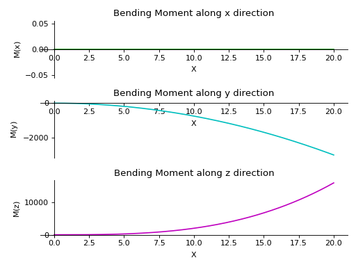
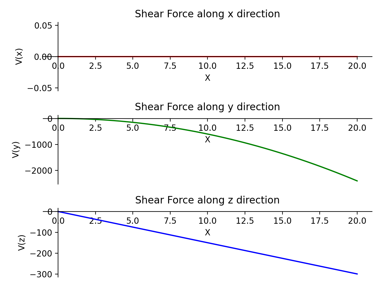
plot_bending_moment(dir='all', subs=None)[source]¶

Returns a plot for bending moment along all three directions present in the Beam object.

Parameters:

dir : string (default

Direction along which bending moment plot is required. If no direction is specified, all plots are displayed.

subs : dictionary

Python dictionary containing Symbols as key and their corresponding values.

Examples

>>> from sympy.physics.continuum_mechanics.beam import Beam3D
>>> from sympy import symbols
>>> l, E, G, I, A, x = symbols('l, E, G, I, A, x')
>>> b = Beam3D(20, E, G, I, A, x)
>>> b.apply_load(15, start=0, order=0, dir="z")
>>> b.apply_load(12*x, start=0, order=0, dir="y")
>>> b.bc_deflection = [(0, [0, 0, 0]), (20, [0, 0, 0])]
>>> R1, R2, R3, R4 = symbols('R1, R2, R3, R4')
>>> b.apply_load(R1, start=0, order=-1, dir="z")
>>> b.apply_load(R2, start=20, order=-1, dir="z")
>>> b.apply_load(R3, start=0, order=-1, dir="y")
>>> b.apply_load(R4, start=20, order=-1, dir="y")
>>> b.solve_for_reaction_loads(R1, R2, R3, R4)
>>> b.plot_bending_moment()
PlotGrid object containing:
Plot[0]:Plot object containing:
[0]: cartesian line: 0 for x over (0.0, 20.0)
Plot[1]:Plot object containing:
[0]: cartesian line: -15*x**2/2 for x over (0.0, 20.0)
Plot[2]:Plot object containing:
[0]: cartesian line: 2*x**3 for x over (0.0, 20.0)

(png, hires.png, pdf)

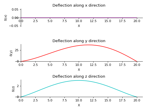
plot_deflection(dir='all', subs=None)[source]¶

Returns a plot for Deflection along all three directions present in the Beam object.

Parameters:

dir : string (default

Direction along which deflection plot is required. If no direction is specified, all plots are displayed.

subs : dictionary

Python dictionary containing Symbols as keys and their corresponding values.

Examples

>>> from sympy.physics.continuum_mechanics.beam import Beam3D
>>> from sympy import symbols
>>> l, E, G, I, A, x = symbols('l, E, G, I, A, x')
>>> b = Beam3D(20, 40, 21, 100, 25, x)
>>> b.apply_load(15, start=0, order=0, dir="z")
>>> b.apply_load(12*x, start=0, order=0, dir="y")
>>> b.bc_deflection = [(0, [0, 0, 0]), (20, [0, 0, 0])]
>>> R1, R2, R3, R4 = symbols('R1, R2, R3, R4')
>>> b.apply_load(R1, start=0, order=-1, dir="z")
>>> b.apply_load(R2, start=20, order=-1, dir="z")
>>> b.apply_load(R3, start=0, order=-1, dir="y")
>>> b.apply_load(R4, start=20, order=-1, dir="y")
>>> b.solve_for_reaction_loads(R1, R2, R3, R4)
>>> b.solve_slope_deflection()
>>> b.plot_deflection()
PlotGrid object containing:
Plot[0]:Plot object containing:
[0]: cartesian line: 0 for x over (0.0, 20.0)
Plot[1]:Plot object containing:
[0]: cartesian line: x**5/40000 - 4013*x**3/90300 + 26*x**2/43 + 1520*x/903 for x over (0.0, 20.0)
Plot[2]:Plot object containing:
[0]: cartesian line: x**4/6400 - x**3/160 + 27*x**2/560 + 2*x/7 for x over (0.0, 20.0)

(png, hires.png, pdf)

plot_loading_results(dir='x', subs=None)[source]¶

Returns a subplot of Shear Force, Bending Moment, Slope and Deflection of the Beam object along the direction specified.

Parameters:

dir : string (default

Direction along which plots are required. If no direction is specified, plots along x-axis are displayed.

subs : dictionary

Python dictionary containing Symbols as key and their corresponding values.

Examples

>>> from sympy.physics.continuum_mechanics.beam import Beam3D
>>> from sympy import symbols
>>> l, E, G, I, A, x = symbols('l, E, G, I, A, x')
>>> b = Beam3D(20, E, G, I, A, x)
>>> subs = {E:40, G:21, I:100, A:25}
>>> b.apply_load(15, start=0, order=0, dir="z")
>>> b.apply_load(12*x, start=0, order=0, dir="y")
>>> b.bc_deflection = [(0, [0, 0, 0]), (20, [0, 0, 0])]
>>> R1, R2, R3, R4 = symbols('R1, R2, R3, R4')
>>> b.apply_load(R1, start=0, order=-1, dir="z")
>>> b.apply_load(R2, start=20, order=-1, dir="z")
>>> b.apply_load(R3, start=0, order=-1, dir="y")
>>> b.apply_load(R4, start=20, order=-1, dir="y")
>>> b.solve_for_reaction_loads(R1, R2, R3, R4)
>>> b.solve_slope_deflection()
>>> b.plot_loading_results('y',subs)
PlotGrid object containing:
Plot[0]:Plot object containing:
[0]: cartesian line: -6*x**2 for x over (0.0, 20.0)
Plot[1]:Plot object containing:
[0]: cartesian line: -15*x**2/2 for x over (0.0, 20.0)
Plot[2]:Plot object containing:
[0]: cartesian line: -x**3/1600 + 3*x**2/160 - x/8 for x over (0.0, 20.0)
Plot[3]:Plot object containing:
[0]: cartesian line: x**5/40000 - 4013*x**3/90300 + 26*x**2/43 + 1520*x/903 for x over (0.0, 20.0)

(png, hires.png, pdf)

plot_shear_force(dir='all', subs=None)[source]¶

Returns a plot for Shear force along all three directions present in the Beam object.

Parameters:

dir : string (default

Direction along which shear force plot is required. If no direction is specified, all plots are displayed.

subs : dictionary

Python dictionary containing Symbols as key and their corresponding values.

Examples

>>> from sympy.physics.continuum_mechanics.beam import Beam3D
>>> from sympy import symbols
>>> l, E, G, I, A, x = symbols('l, E, G, I, A, x')
>>> b = Beam3D(20, E, G, I, A, x)
>>> b.apply_load(15, start=0, order=0, dir="z")
>>> b.apply_load(12*x, start=0, order=0, dir="y")
>>> b.bc_deflection = [(0, [0, 0, 0]), (20, [0, 0, 0])]
>>> R1, R2, R3, R4 = symbols('R1, R2, R3, R4')
>>> b.apply_load(R1, start=0, order=-1, dir="z")
>>> b.apply_load(R2, start=20, order=-1, dir="z")
>>> b.apply_load(R3, start=0, order=-1, dir="y")
>>> b.apply_load(R4, start=20, order=-1, dir="y")
>>> b.solve_for_reaction_loads(R1, R2, R3, R4)
>>> b.plot_shear_force()
PlotGrid object containing:
Plot[0]:Plot object containing:
[0]: cartesian line: 0 for x over (0.0, 20.0)
Plot[1]:Plot object containing:
[0]: cartesian line: -6*x**2 for x over (0.0, 20.0)
Plot[2]:Plot object containing:
[0]: cartesian line: -15*x for x over (0.0, 20.0)

(png, hires.png, pdf)

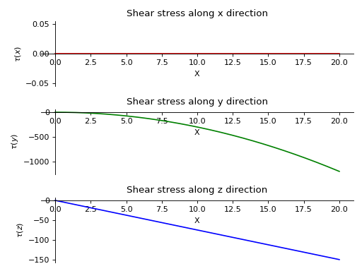
plot_shear_stress(dir='all', subs=None)[source]¶

Returns a plot for Shear Stress along all three directions present in the Beam object.

Parameters:

dir : string (default

Direction along which shear stress plot is required. If no direction is specified, all plots are displayed.

subs : dictionary

Python dictionary containing Symbols as key and their corresponding values.

Examples

There is a beam of length 20 meters and area of cross section 2 square meters. It is supported by rollers at both of its ends. A linear load having slope equal to 12 is applied along y-axis. A constant distributed load of magnitude 15 N is applied from start till its end along z-axis.

>>> from sympy.physics.continuum_mechanics.beam import Beam3D
>>> from sympy import symbols
>>> l, E, G, I, A, x = symbols('l, E, G, I, A, x')
>>> b = Beam3D(20, E, G, I, 2, x)
>>> b.apply_load(15, start=0, order=0, dir="z")
>>> b.apply_load(12*x, start=0, order=0, dir="y")
>>> b.bc_deflection = [(0, [0, 0, 0]), (20, [0, 0, 0])]
>>> R1, R2, R3, R4 = symbols('R1, R2, R3, R4')
>>> b.apply_load(R1, start=0, order=-1, dir="z")
>>> b.apply_load(R2, start=20, order=-1, dir="z")
>>> b.apply_load(R3, start=0, order=-1, dir="y")
>>> b.apply_load(R4, start=20, order=-1, dir="y")
>>> b.solve_for_reaction_loads(R1, R2, R3, R4)
>>> b.plot_shear_stress()
PlotGrid object containing:
Plot[0]:Plot object containing:
[0]: cartesian line: 0 for x over (0.0, 20.0)
Plot[1]:Plot object containing:
[0]: cartesian line: -3*x**2 for x over (0.0, 20.0)
Plot[2]:Plot object containing:
[0]: cartesian line: -15*x/2 for x over (0.0, 20.0)

(png, hires.png, pdf)

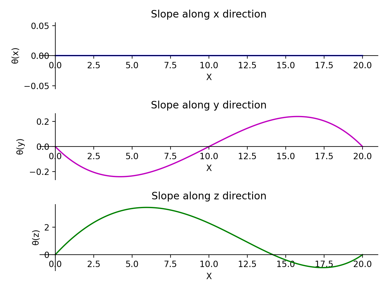
plot_slope(dir='all', subs=None)[source]¶

Returns a plot for Slope along all three directions present in the Beam object.

Parameters:

dir : string (default

Direction along which Slope plot is required. If no direction is specified, all plots are displayed.

subs : dictionary

Python dictionary containing Symbols as keys and their corresponding values.

Examples

>>> from sympy.physics.continuum_mechanics.beam import Beam3D
>>> from sympy import symbols
>>> l, E, G, I, A, x = symbols('l, E, G, I, A, x')
>>> b = Beam3D(20, 40, 21, 100, 25, x)
>>> b.apply_load(15, start=0, order=0, dir="z")
>>> b.apply_load(12*x, start=0, order=0, dir="y")
>>> b.bc_deflection = [(0, [0, 0, 0]), (20, [0, 0, 0])]
>>> R1, R2, R3, R4 = symbols('R1, R2, R3, R4')
>>> b.apply_load(R1, start=0, order=-1, dir="z")
>>> b.apply_load(R2, start=20, order=-1, dir="z")
>>> b.apply_load(R3, start=0, order=-1, dir="y")
>>> b.apply_load(R4, start=20, order=-1, dir="y")
>>> b.solve_for_reaction_loads(R1, R2, R3, R4)
>>> b.solve_slope_deflection()
>>> b.plot_slope()
PlotGrid object containing:
Plot[0]:Plot object containing:
[0]: cartesian line: 0 for x over (0.0, 20.0)
Plot[1]:Plot object containing:
[0]: cartesian line: -x**3/1600 + 3*x**2/160 - x/8 for x over (0.0, 20.0)
Plot[2]:Plot object containing:
[0]: cartesian line: x**4/8000 - 19*x**2/172 + 52*x/43 for x over (0.0, 20.0)

(png, hires.png, pdf)

polar_moment()[source]¶

Returns the polar moment of area of the beam about the X axis with respect to the centroid.

Examples

>>> from sympy.physics.continuum_mechanics.beam import Beam3D
>>> from sympy import symbols
>>> l, E, G, I, A = symbols('l, E, G, I, A')
>>> b = Beam3D(l, E, G, I, A)
>>> b.polar_moment()
2*I
>>> I1 = [9, 15]
>>> b = Beam3D(l, E, G, I1, A)
>>> b.polar_moment()
24

property second_moment¶: Second moment of area of the Beam.

shear_force()[source]¶: Returns a list of three expressions which represents the shear force curve of the Beam object along all three axes.

property shear_modulus¶: Young’s Modulus of the Beam.

shear_stress()[source]¶: Returns a list of three expressions which represents the shear stress curve of the Beam object along all three axes.

slope()[source]¶: Returns a three element list representing slope of deflection curve along all the three axes.

solve_for_reaction_loads(*reaction)[source]¶

Solves for the reaction forces.

Examples

There is a beam of length 30 meters. It it supported by rollers at of its end. A constant distributed load of magnitude 8 N is applied from start till its end along y-axis. Another linear load having slope equal to 9 is applied along z-axis.

>>> from sympy.physics.continuum_mechanics.beam import Beam3D
>>> from sympy import symbols
>>> l, E, G, I, A, x = symbols('l, E, G, I, A, x')
>>> b = Beam3D(30, E, G, I, A, x)
>>> b.apply_load(8, start=0, order=0, dir="y")
>>> b.apply_load(9*x, start=0, order=0, dir="z")
>>> b.bc_deflection = [(0, [0, 0, 0]), (30, [0, 0, 0])]
>>> R1, R2, R3, R4 = symbols('R1, R2, R3, R4')
>>> b.apply_load(R1, start=0, order=-1, dir="y")
>>> b.apply_load(R2, start=30, order=-1, dir="y")
>>> b.apply_load(R3, start=0, order=-1, dir="z")
>>> b.apply_load(R4, start=30, order=-1, dir="z")
>>> b.solve_for_reaction_loads(R1, R2, R3, R4)
>>> b.reaction_loads
{R1: -120, R2: -120, R3: -1350, R4: -2700}

solve_for_torsion()[source]¶

Solves for the angular deflection due to the torsional effects of moments being applied in the x-direction i.e. out of or into the beam.

Here, a positive torque means the direction of the torque is positive i.e. out of the beam along the beam-axis. Likewise, a negative torque signifies a torque into the beam cross-section.

Examples

>>> from sympy.physics.continuum_mechanics.beam import Beam3D
>>> from sympy import symbols
>>> l, E, G, I, A, x = symbols('l, E, G, I, A, x')
>>> b = Beam3D(20, E, G, I, A, x)
>>> b.apply_moment_load(4, 4, -2, dir='x')
>>> b.apply_moment_load(4, 8, -2, dir='x')
>>> b.apply_moment_load(4, 8, -2, dir='x')
>>> b.solve_for_torsion()
>>> b.angular_deflection().subs(x, 3)
18/(G*I)

torsional_moment()[source]¶: Returns expression of Torsional moment present inside the Beam object.