>>> s,k=symbols('s k')>>> gain=k# Let unknown gain be k>>> a=[-3]# Zero at -3 in S plane>>> b=[-1,-2-I,-2+I]# Poles at -1, (-2, j) and (-2, -j) in S plane>>> tf=TransferFunction.from_zpk(a,b,gain,s)>>> pprint(tf) k*(s + 3)-------------------------------(s + 1)*(s + 2 - I)*(s + 2 + I)>>> gain=tf.dc_gain()>>> print(gain)3*k*(2 - I)*(2 + I)/25>>> K=solve(gain-20,k)[0]# Solve for k>>> tf=tf.subs({k:K})# Reconstruct the TransferFunction using .subs()>>> pprint(tf.expand()) 100*s ----- + 100 3------------------- 3 2s + 5*s + 9*s + 5
Subpart 2
>>> tf.is_stable()# Expect True, since poles lie in the left half of S planeTrue
Subpart 3
>>> fromsympyimportinverse_laplace_transform>>> t=symbols('t',positive=True)>>> # Convert from S to T domain for impulse response>>> tf=tf.to_expr()>>> Impulse_Response=inverse_laplace_transform(tf,s,t)>>> pprint(Impulse_Response) -t -2*t 100*e 100*e *cos(t) ------- - ---------------- 3 3
Subpart 4
>>> # Apply the Initial Value Theorem on Equation of S domain>>> # limit(y(t), t, 0) = limit(s*Y(S), s, oo)>>> limit(s*tf,s,oo)0
>>> f=m*diff(y(t),t,t)+c*diff(y(t),t)+k*y(t)-u(t)>>> F=laplace_transform(f,t,s,noconds=True)>>> F=laplace_correspondence(F,{u:U,y:Y})>>> F=laplace_initial_conds(F,t,{y:[0,0]})>>> t=(solve(F,Y(s))[0])/U(s)# To construct Transfer Function from Y(s) and U(s)>>> tf=TransferFunction.from_rational_expression(t,s)>>> pprint(tf) 1-------------- 2c*s + k + m*s
The system matrix (Transfer Function Matrix) in the Laplace domain (g(t) → G(s)).
The number of input and output signals in the system.
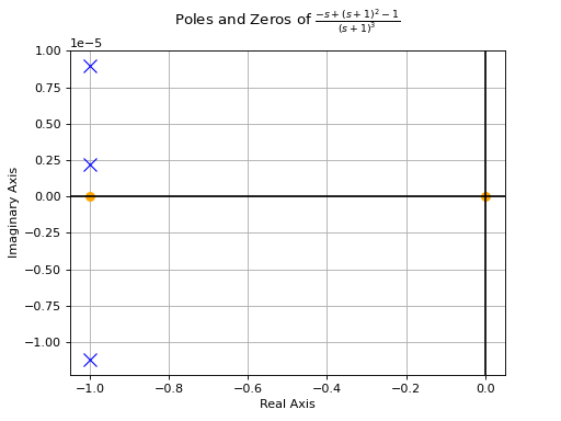
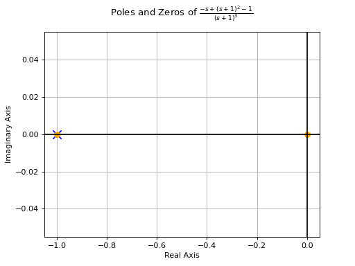
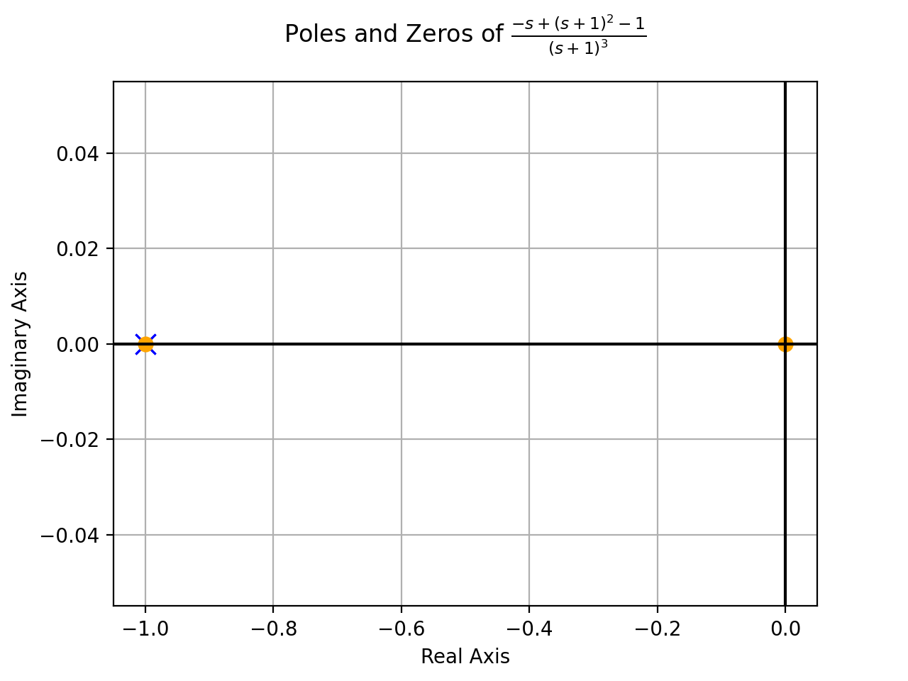
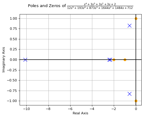
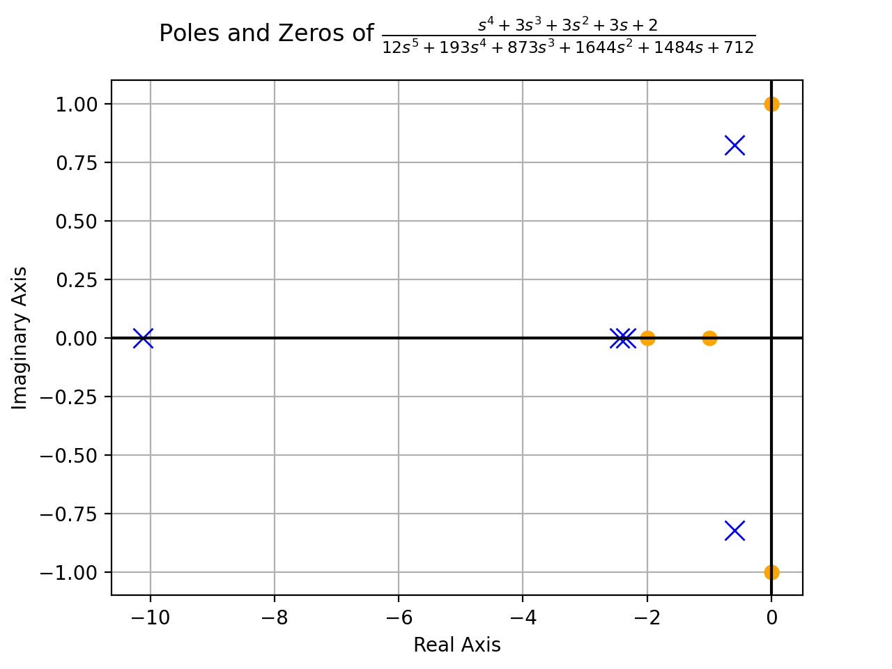
Poles and Zeros of the system elements (individual Transfer Functions in Transfer Function Matrix) in the Laplace domain (Note: The actual poles and zeros of a MIMO system are NOT the poles and zeros of the individual elements of the transfer function matrix). Also, visualise the poles and zeros of the individual transfer function corresponding to the 1st input and 1st output of the G(s) matrix.
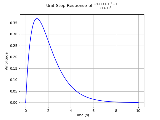
Plot the unit step response of the individual Transfer Function corresponding to the 1st input and 1st output of the G(s) matrix.
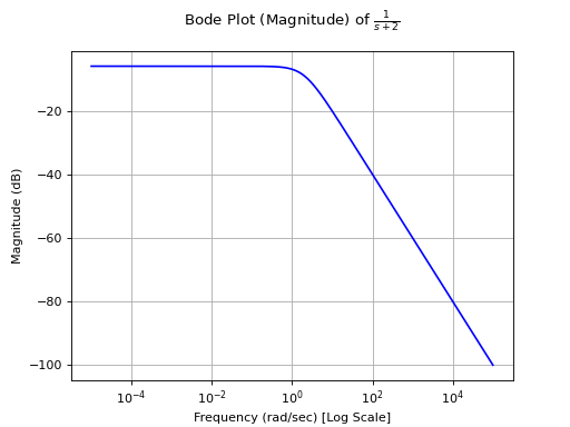
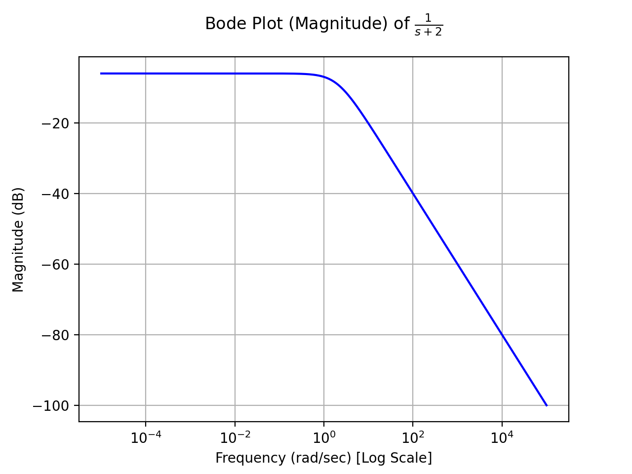
Analyse the Bode magnitude and phase plot of the Transfer Function corresponding to 1st input and 2nd output of the G(s) matrix.
A system is designed by arranging P(s) and C(s) in a series configuration (Values of P(s) and C(s) are provided below). Compute the equivalent system matrix, when the order of blocks is reversed (i.e. C(s) then P(s)).
Also, find the equivalent closed-loop system(or the ratio v/u from the block diagram given below) for the system (negative-feedback loop) having C(s) as the controller and P(s) as plant(Refer to the block diagram given below).
1. The transfer function \(W(z)\) from input \(r(k)\) to output
\(y(k)\).
2. Determine a finite-duration input signal \(u(k)\) (i.e., such that there
exists an \(h \in \mathbb{N}\) for which \(u(k) = 0\) for all
\(k \geq h\)) so that the resulting forced response \(y_f(k)\) converges
to zero.
Solution
>>> # Imports>>> fromsympyimport*>>> fromsympy.abcimportz>>> fromsympy.physics.controlimport*>>> # Transfer function definitions>>> G1=DiscreteTransferFunction(z,z-Rational(1,2),z)>>> G2=DiscreteTransferFunction(z,z-1,z)>>> G3=DiscreteTransferFunction(1,z,z)
Subpart 1
>>> W_partial=Feedback(G1,G3)*G2# the operator * is used for Series connection>>> W=Feedback(W_partial,G3)>>> W=W.doit().to_standard_form(cancel_poles_zeros=True)>>> pprint(W,use_unicode=False) 2 2*z------------ [st: 1] 22*z + z - 1
Subpart 2
First of all we need to study the poles and the stability of the system.
>>> W.poles()[-1, 1/2]>>> W.is_stable()False
The system is not asymptotically stable, so we need to find a
finite-duration input signal \(u(k)\) such that the pole in
\(-1\) is cancelled out.
\[Y(z) = W(z) \cdot U(z)\]
In the numerator of U(z) we need \((z + 1)\) as a factor, and in the
denominator we need something that permits \(u(k)\) to be
finite-duration.
A simple solution is:
\[U(z) = \frac{z + 1}{z}\]
as \(u(k) = \delta(k) + \delta(k - 1)\)
We can check that the output is asymptotically stable:
1. Determine the forced response in the output \(y_f(k)\) with respect to the inputs \(u_1(k)=\theta(k)\) and \(u_2(k) = 0\ \forall k\).
(\(\theta(k)\) represent the heaviside function).
We know that the heaviside function \(\theta(k)\) has the following Z-transform:
\[\theta(z) = \frac{z}{z - 1}\]
So, we can define the input as follows:
>>> U1=z/(z-1)
The forced response in the output is given by:
\[Y_f(z) = G(z) \cdot U(z)\]
where \(G(z)\) is the transfer function associated to the state-space representation
ss and \(U(z)\) is \([\frac{z}{z - 1}, 0]^T\).
(Since \(U_2(z) = 0\), we can consider only the first column of \(G(z)\)).


 >>> bode_phase_plot(tf2)


