Plotting

Introduction

The plotting module allows you to make 2-dimensional and 3-dimensional plots. Presently the plots are rendered using matplotlib as a backend. It is also possible to plot 2-dimensional plots using a TextBackend if you do not have matplotlib.

The plotting module has the following functions:

• plot(): Plots 2D line plots.

• plot_parametric(): Plots 2D parametric plots.

• plot_implicit(): Plots 2D implicit and region plots.

• plot3d(): Plots 3D plots of functions in two variables.

• plot3d_parametric_line(): Plots 3D line plots, defined by a parameter.

• plot3d_parametric_surface(): Plots 3D parametric surface plots.

The above functions are only for convenience and ease of use. It is possible to plot any plot by passing the corresponding Series class to Plot as argument.

Plot Class

class sympy.plotting.plot.Plot(

*args,

title=None,

xlabel=None,

ylabel=None,

zlabel=None,

aspect_ratio='auto',

xlim=None,

ylim=None,

axis_center='auto',

axis=True,

xscale='linear',

yscale='linear',

legend=False,

autoscale=True,

margin=0,

annotations=None,

markers=None,

rectangles=None,

fill=None,

backend='default',

size=None,

**kwargs,

)

Base class for all backends. A backend represents the plotting library, which implements the necessary functionalities in order to use SymPy plotting functions.

For interactive work the function plot() is better suited.

This class permits the plotting of SymPy expressions using numerous backends (matplotlib, textplot, the old pyglet module for SymPy, Google charts api, etc).

The figure can contain an arbitrary number of plots of SymPy expressions, lists of coordinates of points, etc. Plot has a private attribute _series that contains all data series to be plotted (expressions for lines or surfaces, lists of points, etc (all subclasses of BaseSeries)). Those data series are instances of classes not imported by from sympy import *.

The customization of the figure is on two levels. Global options that concern the figure as a whole (e.g. title, xlabel, scale, etc) and per-data series options (e.g. name) and aesthetics (e.g. color, point shape, line type, etc.).

The difference between options and aesthetics is that an aesthetic can be a function of the coordinates (or parameters in a parametric plot). The supported values for an aesthetic are:

• None (the backend uses default values)

• a constant

• a function of one variable (the first coordinate or parameter)

• a function of two variables (the first and second coordinate or parameters)

• a function of three variables (only in nonparametric 3D plots)

Their implementation depends on the backend so they may not work in some backends.

If the plot is parametric and the arity of the aesthetic function permits it the aesthetic is calculated over parameters and not over coordinates. If the arity does not permit calculation over parameters the calculation is done over coordinates.

Only cartesian coordinates are supported for the moment, but you can use the parametric plots to plot in polar, spherical and cylindrical coordinates.

The arguments for the constructor Plot must be subclasses of BaseSeries.

Any global option can be specified as a keyword argument.

The global options for a figure are:

• title : str

• xlabel : str or Symbol

• ylabel : str or Symbol

• zlabel : str or Symbol

• legend : bool

• xscale : {‘linear’, ‘log’}

• yscale : {‘linear’, ‘log’}

• axis : bool

• axis_center : tuple of two floats or {‘center’, ‘auto’}

• xlim : tuple of two floats

• ylim : tuple of two floats

• aspect_ratio : tuple of two floats or {‘auto’}

• autoscale : bool

• margin : float in [0, 1]

• backend : {‘default’, ‘matplotlib’, ‘text’} or a subclass of BaseBackend

• size : optional tuple of two floats, (width, height); default: None

The per data series options and aesthetics are: There are none in the base series. See below for options for subclasses.

Some data series support additional aesthetics or options:

LineOver1DRangeSeries, Parametric2DLineSeries, and Parametric3DLineSeries support the following:

Aesthetics:

• line_colorstring, or float, or function, optional

  Specifies the color for the plot, which depends on the backend being used.

  For example, if MatplotlibBackend is being used, then Matplotlib string colors are acceptable ("red", "r", "cyan", "c", …). Alternatively, we can use a float number, 0 < color < 1, wrapped in a string (for example, line_color="0.5") to specify grayscale colors. Alternatively, We can specify a function returning a single float value: this will be used to apply a color-loop (for example, line_color=lambda x: math.cos(x)).

  Note that by setting line_color, it would be applied simultaneously to all the series.

Options:

• label : str

• steps : bool

• integers_only : bool

SurfaceOver2DRangeSeries and ParametricSurfaceSeries support the following:

Aesthetics:

• surface_color : function which returns a float.

Notes

How the plotting module works:

1. Whenever a plotting function is called, the provided expressions are processed and a list of instances of the BaseSeries class is created, containing the necessary information to plot the expressions (e.g. the expression, ranges, series name, …). Eventually, these objects will generate the numerical data to be plotted.

2. A subclass of Plot class is instantiaed (referred to as backend, from now on), which stores the list of series and the main attributes of the plot (e.g. axis labels, title, …). The backend implements the logic to generate the actual figure with some plotting library.

3. When the show command is executed, series are processed one by one to generate numerical data and add it to the figure. The backend is also going to set the axis labels, title, …, according to the values stored in the Plot instance.

The backend should check if it supports the data series that it is given (e.g. TextBackend supports only LineOver1DRangeSeries).

It is the backend responsibility to know how to use the class of data series that it’s given. Note that the current implementation of the *Series classes is “matplotlib-centric”: the numerical data returned by the get_points and get_meshes methods is meant to be used directly by Matplotlib. Therefore, the new backend will have to pre-process the numerical data to make it compatible with the chosen plotting library. Keep in mind that future SymPy versions may improve the *Series classes in order to return numerical data “non-matplotlib-centric”, hence if you code a new backend you have the responsibility to check if its working on each SymPy release.

Please explore the MatplotlibBackend source code to understand how a backend should be coded.

In order to be used by SymPy plotting functions, a backend must implement the following methods:

• show(self): used to loop over the data series, generate the numerical

  data, plot it and set the axis labels, title, …

• save(self, path): used to save the current plot to the specified file

  path.

• close(self): used to close the current plot backend (note: some plotting

  library does not support this functionality. In that case, just raise a warning).

property annotations

Deprecated since version 1.13.

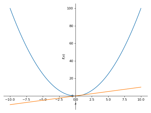
append(arg)

Adds an element from a plot’s series to an existing plot.

Examples

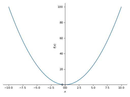
Consider two Plot objects, p1 and p2. To add the second plot’s first series object to the first, use the append method, like so:

>>> from sympy import symbols
>>> from sympy.plotting import plot
>>> x = symbols('x')
>>> p1 = plot(x*x, show=False)
>>> p2 = plot(x, show=False)
>>> p1.append(p2[0])
>>> p1
Plot object containing:
[0]: cartesian line: x**2 for x over (-10.0, 10.0)
[1]: cartesian line: x for x over (-10.0, 10.0)
>>> p1.show()

(png, hires.png, pdf)

See also

extend

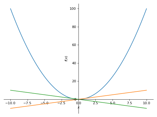
extend(arg)

Adds all series from another plot.

Examples

Consider two Plot objects, p1 and p2. To add the second plot to the first, use the extend method, like so:

>>> from sympy import symbols
>>> from sympy.plotting import plot
>>> x = symbols('x')
>>> p1 = plot(x**2, show=False)
>>> p2 = plot(x, -x, show=False)
>>> p1.extend(p2)
>>> p1
Plot object containing:
[0]: cartesian line: x**2 for x over (-10.0, 10.0)
[1]: cartesian line: x for x over (-10.0, 10.0)
[2]: cartesian line: -x for x over (-10.0, 10.0)
>>> p1.show()

(png, hires.png, pdf)

property fill

Deprecated since version 1.13.

property markers

Deprecated since version 1.13.

property rectangles

Deprecated since version 1.13.

Plotting Function Reference

sympy.plotting.plot.plot(*args, show=True, **kwargs)

Plots a function of a single variable as a curve.

Parameters:

args :

The first argument is the expression representing the function of single variable to be plotted.

The last argument is a 3-tuple denoting the range of the free variable. e.g. (x, 0, 5)

Typical usage examples are in the following:

• Plotting a single expression with a single range.

  plot(expr, range, **kwargs)

• Plotting a single expression with the default range (-10, 10).

  plot(expr, **kwargs)

• Plotting multiple expressions with a single range.

  plot(expr1, expr2, ..., range, **kwargs)

• Plotting multiple expressions with multiple ranges.

  plot((expr1, range1), (expr2, range2), ..., **kwargs)

It is best practice to specify range explicitly because default range may change in the future if a more advanced default range detection algorithm is implemented.

show : bool, optional

The default value is set to True. Set show to False and the function will not display the plot. The returned instance of the Plot class can then be used to save or display the plot by calling the save() and show() methods respectively.

line_color : string, or float, or function, optional

Specifies the color for the plot. See Plot to see how to set color for the plots. Note that by setting line_color, it would be applied simultaneously to all the series.

title : str, optional

Title of the plot. It is set to the latex representation of the expression, if the plot has only one expression.

label : str, optional

The label of the expression in the plot. It will be used when called with legend. Default is the name of the expression. e.g. sin(x)

xlabel : str or expression, optional

Label for the x-axis.

ylabel : str or expression, optional

Label for the y-axis.

xscale : ‘linear’ or ‘log’, optional

Sets the scaling of the x-axis.

yscale : ‘linear’ or ‘log’, optional

Sets the scaling of the y-axis.

axis_center : (float, float), optional

Tuple of two floats denoting the coordinates of the center or {‘center’, ‘auto’}

xlim : (float, float), optional

Denotes the x-axis limits, (min, max)`.

ylim : (float, float), optional

Denotes the y-axis limits, (min, max)`.

annotations : list, optional

A list of dictionaries specifying the type of annotation required. The keys in the dictionary should be equivalent to the arguments of the matplotlib’s annotate() method.

markers : list, optional

A list of dictionaries specifying the type the markers required. The keys in the dictionary should be equivalent to the arguments of the matplotlib’s plot() function along with the marker related keyworded arguments.

rectangles : list, optional

A list of dictionaries specifying the dimensions of the rectangles to be plotted. The keys in the dictionary should be equivalent to the arguments of the matplotlib’s Rectangle class.

fill : dict, optional

A dictionary specifying the type of color filling required in the plot. The keys in the dictionary should be equivalent to the arguments of the matplotlib’s fill_between() method.

adaptive : bool, optional

The default value is set to True. Set adaptive to False and specify n if uniform sampling is required.

The plotting uses an adaptive algorithm which samples recursively to accurately plot. The adaptive algorithm uses a random point near the midpoint of two points that has to be further sampled. Hence the same plots can appear slightly different.

depth : int, optional

Recursion depth of the adaptive algorithm. A depth of value \(n\) samples a maximum of \(2^{n}\) points.

If the adaptive flag is set to False, this will be ignored.

n : int, optional

Used when the adaptive is set to False. The function is uniformly sampled at n number of points. If the adaptive flag is set to True, this will be ignored. This keyword argument replaces nb_of_points, which should be considered deprecated.

size : (float, float), optional

A tuple in the form (width, height) in inches to specify the size of the overall figure. The default value is set to None, meaning the size will be set by the default backend.

Examples

>>> from sympy import symbols
>>> from sympy.plotting import plot
>>> x = symbols('x')

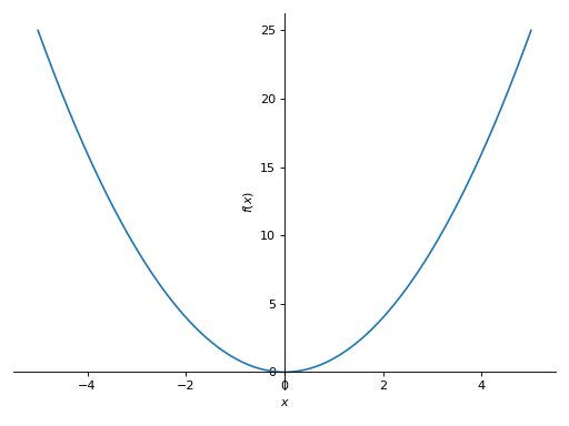
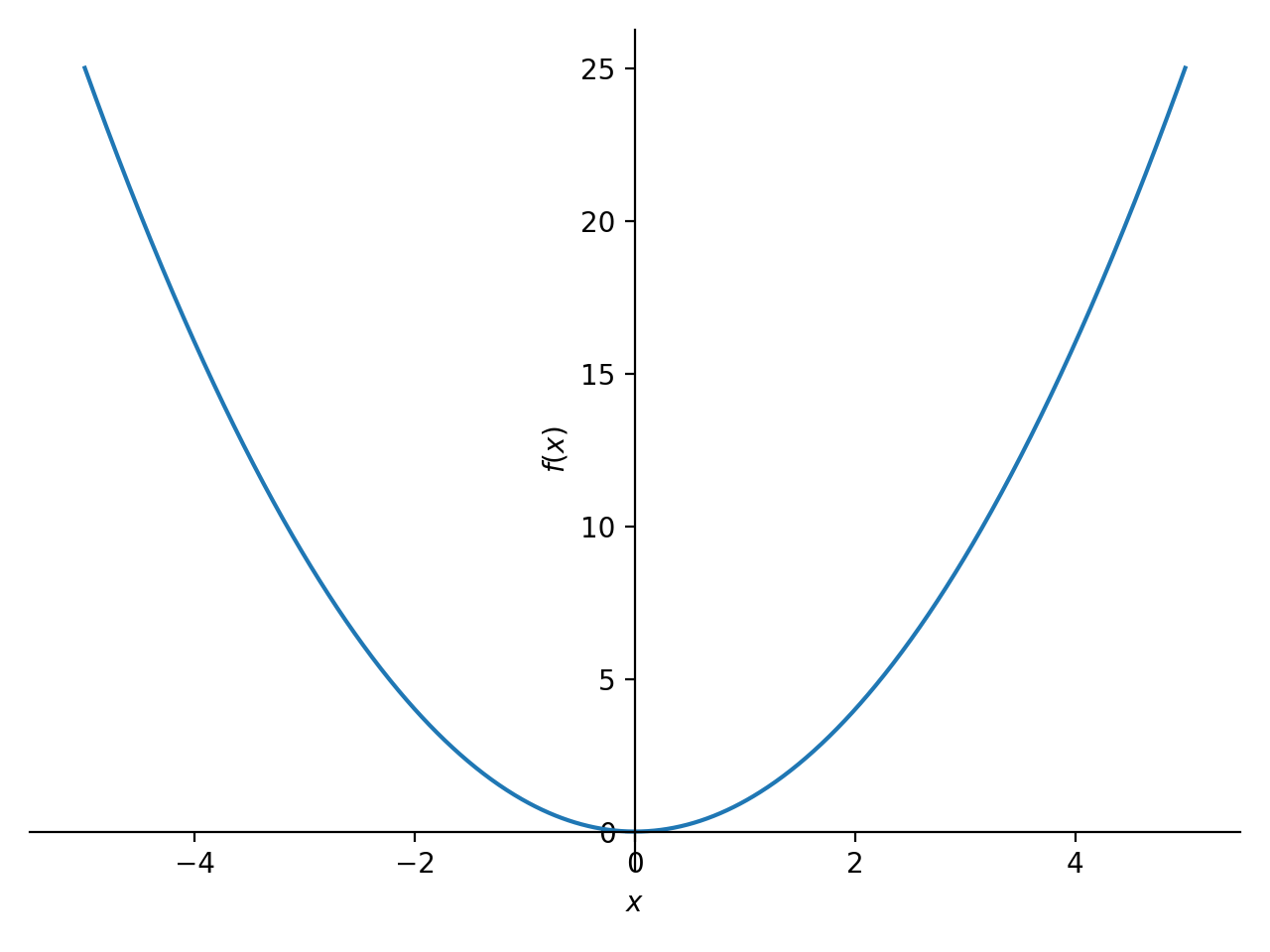
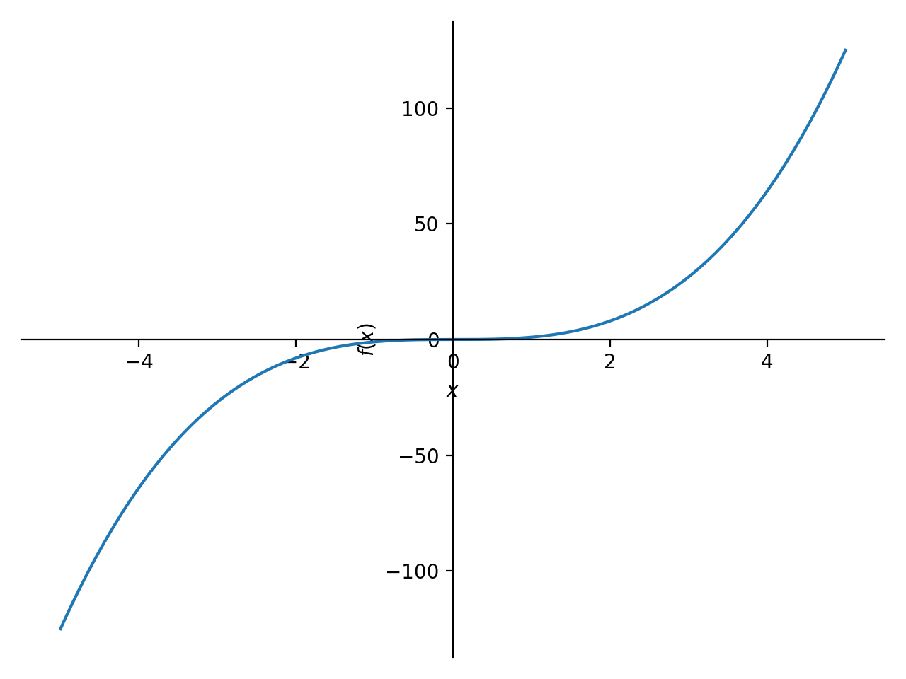
Single Plot

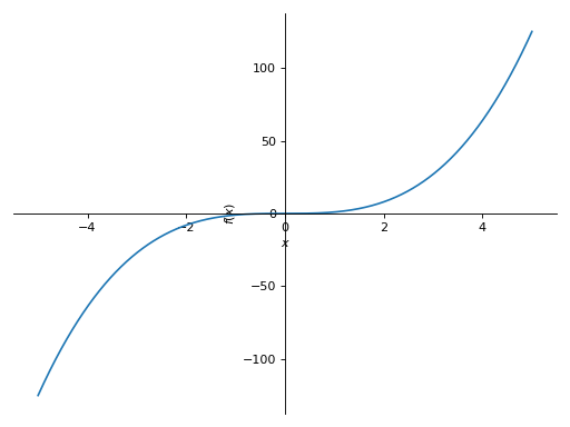
>>> plot(x**2, (x, -5, 5))
Plot object containing:
[0]: cartesian line: x**2 for x over (-5.0, 5.0)

(png, hires.png, pdf)

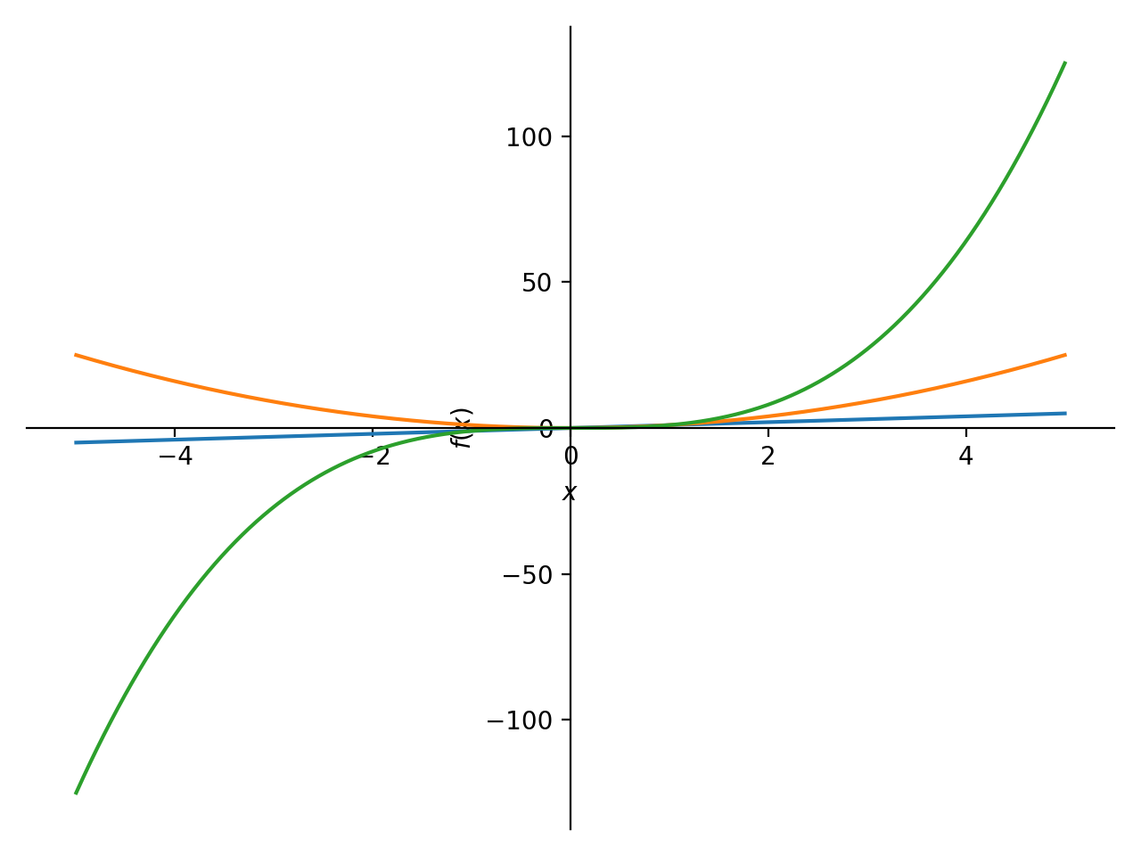
Multiple plots with single range.

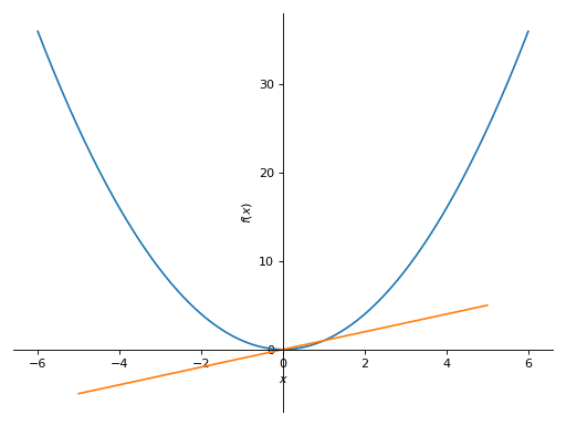
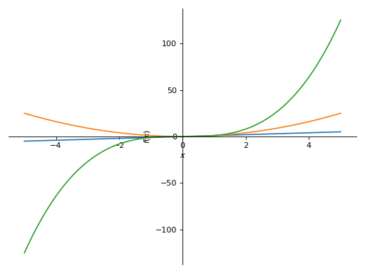
>>> plot(x, x**2, x**3, (x, -5, 5))
Plot object containing:
[0]: cartesian line: x for x over (-5.0, 5.0)
[1]: cartesian line: x**2 for x over (-5.0, 5.0)
[2]: cartesian line: x**3 for x over (-5.0, 5.0)

(png, hires.png, pdf)

Multiple plots with different ranges.

>>> plot((x**2, (x, -6, 6)), (x, (x, -5, 5)))
Plot object containing:
[0]: cartesian line: x**2 for x over (-6.0, 6.0)
[1]: cartesian line: x for x over (-5.0, 5.0)

(png, hires.png, pdf)

No adaptive sampling.

>>> plot(x**2, adaptive=False, n=400)
Plot object containing:
[0]: cartesian line: x**2 for x over (-10.0, 10.0)

(png, hires.png, pdf)

See also

Plot, LineOver1DRangeSeries

sympy.plotting.plot.plot_parametric(*args, show=True, **kwargs)

Plots a 2D parametric curve.

Parameters:

args

Common specifications are:

• Plotting a single parametric curve with a range

  plot_parametric((expr_x, expr_y), range)

• Plotting multiple parametric curves with the same range

  plot_parametric((expr_x, expr_y), ..., range)

• Plotting multiple parametric curves with different ranges

  plot_parametric((expr_x, expr_y, range), ...)

expr_x is the expression representing \(x\) component of the parametric function.

expr_y is the expression representing \(y\) component of the parametric function.

range is a 3-tuple denoting the parameter symbol, start and stop. For example, (u, 0, 5).

If the range is not specified, then a default range of (-10, 10) is used.

However, if the arguments are specified as (expr_x, expr_y, range), ..., you must specify the ranges for each expressions manually.

Default range may change in the future if a more advanced algorithm is implemented.

adaptive : bool, optional

Specifies whether to use the adaptive sampling or not.

The default value is set to True. Set adaptive to False and specify n if uniform sampling is required.

depth : int, optional

The recursion depth of the adaptive algorithm. A depth of value \(n\) samples a maximum of \(2^n\) points.

n : int, optional

Used when the adaptive flag is set to False. Specifies the number of the points used for the uniform sampling. This keyword argument replaces nb_of_points, which should be considered deprecated.

line_color : string, or float, or function, optional

Specifies the color for the plot. See Plot to see how to set color for the plots. Note that by setting line_color, it would be applied simultaneously to all the series.

label : str, optional

The label of the expression in the plot. It will be used when called with legend. Default is the name of the expression. e.g. sin(x)

xlabel : str, optional

Label for the x-axis.

ylabel : str, optional

Label for the y-axis.

xscale : ‘linear’ or ‘log’, optional

Sets the scaling of the x-axis.

yscale : ‘linear’ or ‘log’, optional

Sets the scaling of the y-axis.

axis_center : (float, float), optional

Tuple of two floats denoting the coordinates of the center or {‘center’, ‘auto’}

xlim : (float, float), optional

Denotes the x-axis limits, (min, max)`.

ylim : (float, float), optional

Denotes the y-axis limits, (min, max)`.

size : (float, float), optional

A tuple in the form (width, height) in inches to specify the size of the overall figure. The default value is set to None, meaning the size will be set by the default backend.

Examples

>>> from sympy import plot_parametric, symbols, cos, sin
>>> u = symbols('u')

A parametric plot with a single expression:

>>> plot_parametric((cos(u), sin(u)), (u, -5, 5))
Plot object containing:
[0]: parametric cartesian line: (cos(u), sin(u)) for u over (-5.0, 5.0)

(png, hires.png, pdf)

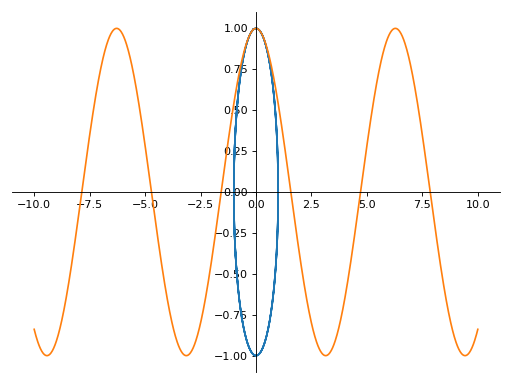
A parametric plot with multiple expressions with the same range:

>>> plot_parametric((cos(u), sin(u)), (u, cos(u)), (u, -10, 10))
Plot object containing:
[0]: parametric cartesian line: (cos(u), sin(u)) for u over (-10.0, 10.0)
[1]: parametric cartesian line: (u, cos(u)) for u over (-10.0, 10.0)

(png, hires.png, pdf)

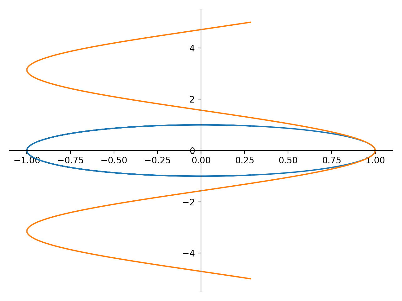
A parametric plot with multiple expressions with different ranges for each curve:

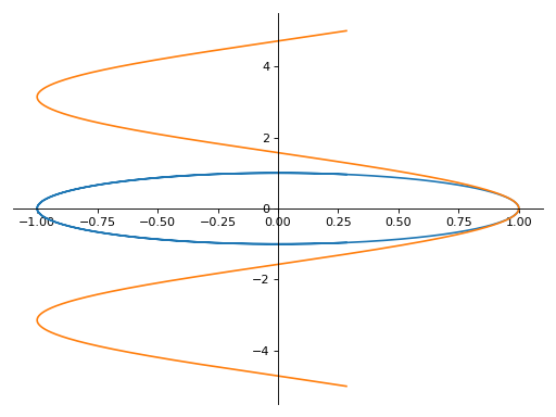
>>> plot_parametric((cos(u), sin(u), (u, -5, 5)),
...     (cos(u), u, (u, -5, 5)))
Plot object containing:
[0]: parametric cartesian line: (cos(u), sin(u)) for u over (-5.0, 5.0)
[1]: parametric cartesian line: (cos(u), u) for u over (-5.0, 5.0)

(png, hires.png, pdf)

Notes

The plotting uses an adaptive algorithm which samples recursively to accurately plot the curve. The adaptive algorithm uses a random point near the midpoint of two points that has to be further sampled. Hence, repeating the same plot command can give slightly different results because of the random sampling.

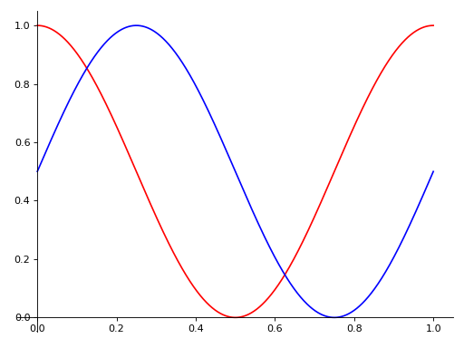
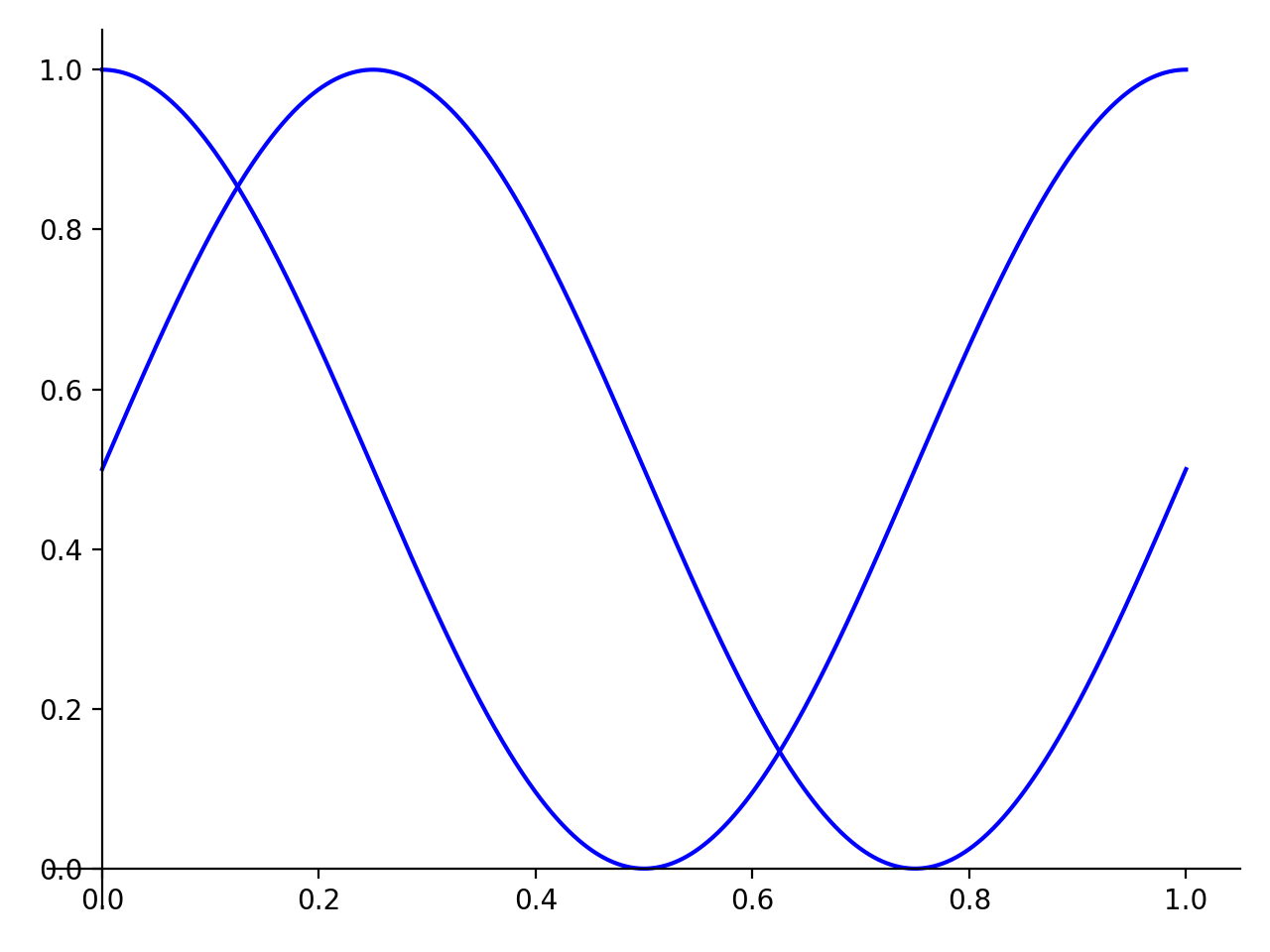
If there are multiple plots, then the same optional arguments are applied to all the plots drawn in the same canvas. If you want to set these options separately, you can index the returned Plot object and set it.

For example, when you specify line_color once, it would be applied simultaneously to both series.

>>> from sympy import pi
>>> expr1 = (u, cos(2*pi*u)/2 + 1/2)
>>> expr2 = (u, sin(2*pi*u)/2 + 1/2)
>>> p = plot_parametric(expr1, expr2, (u, 0, 1), line_color='blue')

(png, hires.png, pdf)

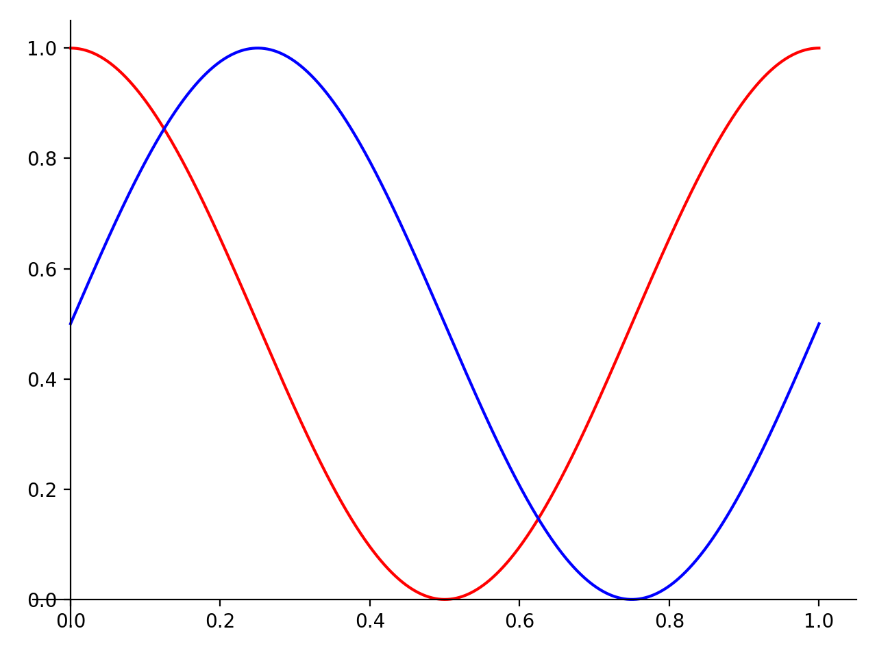
If you want to specify the line color for the specific series, you should index each item and apply the property manually.

>>> p[0].line_color = 'red'
>>> p.show()

(png, hires.png, pdf)

See also

Plot, Parametric2DLineSeries

sympy.plotting.plot.plot3d(*args, show=True, **kwargs)

Plots a 3D surface plot.

Usage

Single plot

plot3d(expr, range_x, range_y, **kwargs)

If the ranges are not specified, then a default range of (-10, 10) is used.

Multiple plot with the same range.

plot3d(expr1, expr2, range_x, range_y, **kwargs)

If the ranges are not specified, then a default range of (-10, 10) is used.

Multiple plots with different ranges.

plot3d((expr1, range_x, range_y), (expr2, range_x, range_y), ..., **kwargs)

Ranges have to be specified for every expression.

Default range may change in the future if a more advanced default range detection algorithm is implemented.

Arguments

expr : Expression representing the function along x.

range_x(Symbol, float, float)

A 3-tuple denoting the range of the x variable, e.g. (x, 0, 5).

range_y(Symbol, float, float)

A 3-tuple denoting the range of the y variable, e.g. (y, 0, 5).

Keyword Arguments

Arguments for SurfaceOver2DRangeSeries class:

n1int

The x range is sampled uniformly at n1 of points. This keyword argument replaces nb_of_points_x, which should be considered deprecated.

n2int

The y range is sampled uniformly at n2 of points. This keyword argument replaces nb_of_points_y, which should be considered deprecated.

Aesthetics:

surface_colorFunction which returns a float

Specifies the color for the surface of the plot. See Plot for more details.

If there are multiple plots, then the same series arguments are applied to all the plots. If you want to set these options separately, you can index the returned Plot object and set it.

Arguments for Plot class:

titlestr

Title of the plot.

size(float, float), optional

A tuple in the form (width, height) in inches to specify the size of the overall figure. The default value is set to None, meaning the size will be set by the default backend.

Examples

>>> from sympy import symbols
>>> from sympy.plotting import plot3d
>>> x, y = symbols('x y')

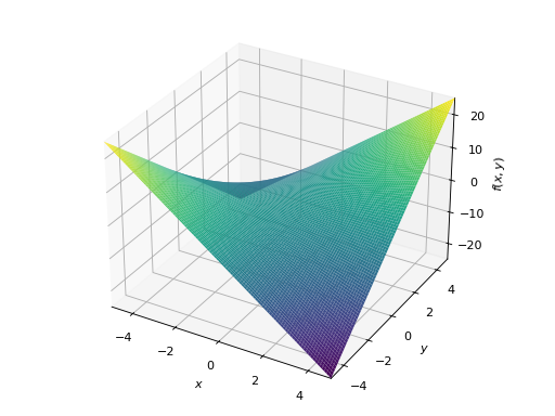
Single plot

>>> plot3d(x*y, (x, -5, 5), (y, -5, 5))
Plot object containing:
[0]: cartesian surface: x*y for x over (-5.0, 5.0) and y over (-5.0, 5.0)

(png, hires.png, pdf)

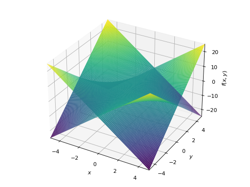
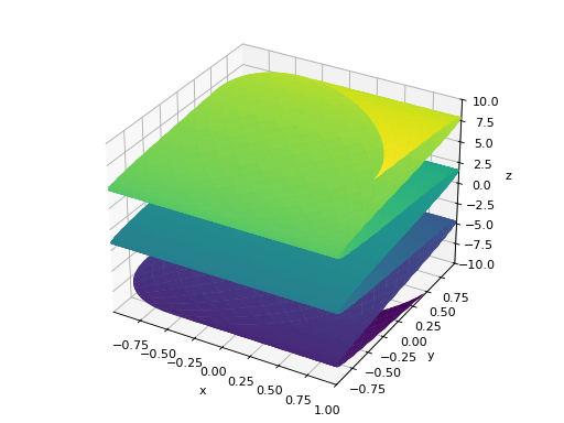
Multiple plots with same range

>>> plot3d(x*y, -x*y, (x, -5, 5), (y, -5, 5))
Plot object containing:
[0]: cartesian surface: x*y for x over (-5.0, 5.0) and y over (-5.0, 5.0)
[1]: cartesian surface: -x*y for x over (-5.0, 5.0) and y over (-5.0, 5.0)

(png, hires.png, pdf)

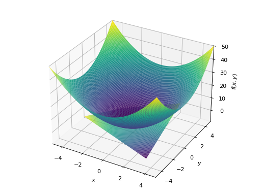
Multiple plots with different ranges.

>>> plot3d((x**2 + y**2, (x, -5, 5), (y, -5, 5)),
...     (x*y, (x, -3, 3), (y, -3, 3)))
Plot object containing:
[0]: cartesian surface: x**2 + y**2 for x over (-5.0, 5.0) and y over (-5.0, 5.0)
[1]: cartesian surface: x*y for x over (-3.0, 3.0) and y over (-3.0, 3.0)

(png, hires.png, pdf)

See also

Plot, SurfaceOver2DRangeSeries

sympy.plotting.plot.plot3d_parametric_line(*args, show=True, **kwargs)

Plots a 3D parametric line plot.

Usage

Single plot:

plot3d_parametric_line(expr_x, expr_y, expr_z, range, **kwargs)

If the range is not specified, then a default range of (-10, 10) is used.

Multiple plots.

plot3d_parametric_line((expr_x, expr_y, expr_z, range), ..., **kwargs)

Ranges have to be specified for every expression.

Default range may change in the future if a more advanced default range detection algorithm is implemented.

Arguments

expr_x : Expression representing the function along x.

expr_y : Expression representing the function along y.

expr_z : Expression representing the function along z.

range(Symbol, float, float)

A 3-tuple denoting the range of the parameter variable, e.g., (u, 0, 5).

Keyword Arguments

Arguments for Parametric3DLineSeries class.

nint

The range is uniformly sampled at n number of points. This keyword argument replaces nb_of_points, which should be considered deprecated.

Aesthetics:

line_colorstring, or float, or function, optional

Specifies the color for the plot. See Plot to see how to set color for the plots. Note that by setting line_color, it would be applied simultaneously to all the series.

labelstr

The label to the plot. It will be used when called with legend=True to denote the function with the given label in the plot.

If there are multiple plots, then the same series arguments are applied to all the plots. If you want to set these options separately, you can index the returned Plot object and set it.

Arguments for Plot class.

titlestr

Title of the plot.

size(float, float), optional

A tuple in the form (width, height) in inches to specify the size of the overall figure. The default value is set to None, meaning the size will be set by the default backend.

Examples

>>> from sympy import symbols, cos, sin
>>> from sympy.plotting import plot3d_parametric_line
>>> u = symbols('u')

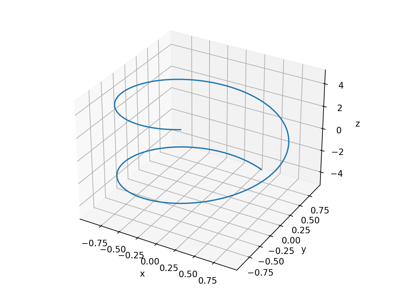
Single plot.

>>> plot3d_parametric_line(cos(u), sin(u), u, (u, -5, 5))
Plot object containing:
[0]: 3D parametric cartesian line: (cos(u), sin(u), u) for u over (-5.0, 5.0)

(png, hires.png, pdf)

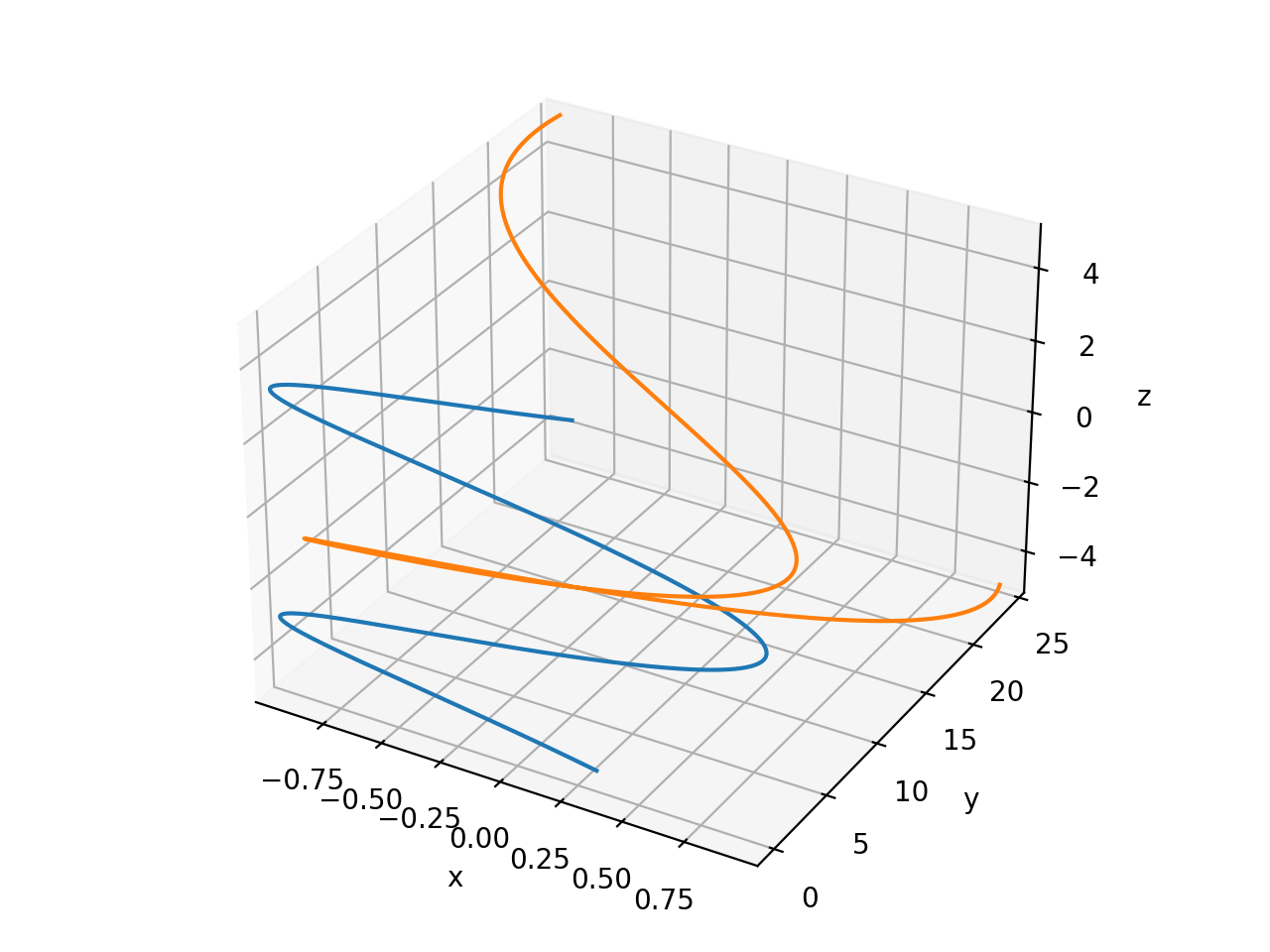
Multiple plots.

>>> plot3d_parametric_line((cos(u), sin(u), u, (u, -5, 5)),
...     (sin(u), u**2, u, (u, -5, 5)))
Plot object containing:
[0]: 3D parametric cartesian line: (cos(u), sin(u), u) for u over (-5.0, 5.0)
[1]: 3D parametric cartesian line: (sin(u), u**2, u) for u over (-5.0, 5.0)

(png, hires.png, pdf)

See also

Plot, Parametric3DLineSeries

sympy.plotting.plot.plot3d_parametric_surface(

*args,

show=True,

**kwargs,

)

Plots a 3D parametric surface plot.

Explanation

Single plot.

plot3d_parametric_surface(expr_x, expr_y, expr_z, range_u, range_v, **kwargs)

If the ranges is not specified, then a default range of (-10, 10) is used.

Multiple plots.

plot3d_parametric_surface((expr_x, expr_y, expr_z, range_u, range_v), ..., **kwargs)

Ranges have to be specified for every expression.

Default range may change in the future if a more advanced default range detection algorithm is implemented.

Arguments

expr_x : Expression representing the function along x.

expr_y : Expression representing the function along y.

expr_z : Expression representing the function along z.

range_u(Symbol, float, float)

A 3-tuple denoting the range of the u variable, e.g. (u, 0, 5).

range_v(Symbol, float, float)

A 3-tuple denoting the range of the v variable, e.g. (v, 0, 5).

Keyword Arguments

Arguments for ParametricSurfaceSeries class:

n1int

The u range is sampled uniformly at n1 of points. This keyword argument replaces nb_of_points_u, which should be considered deprecated.

n2int

The v range is sampled uniformly at n2 of points. This keyword argument replaces nb_of_points_v, which should be considered deprecated.

Aesthetics:

surface_colorFunction which returns a float

Specifies the color for the surface of the plot. See Plot for more details.

If there are multiple plots, then the same series arguments are applied for all the plots. If you want to set these options separately, you can index the returned Plot object and set it.

Arguments for Plot class:

titlestr

Title of the plot.

size(float, float), optional

A tuple in the form (width, height) in inches to specify the size of the overall figure. The default value is set to None, meaning the size will be set by the default backend.

Examples

>>> from sympy import symbols, cos, sin
>>> from sympy.plotting import plot3d_parametric_surface
>>> u, v = symbols('u v')

Single plot.

>>> plot3d_parametric_surface(cos(u + v), sin(u - v), u - v,
...     (u, -5, 5), (v, -5, 5))
Plot object containing:
[0]: parametric cartesian surface: (cos(u + v), sin(u - v), u - v) for u over (-5.0, 5.0) and v over (-5.0, 5.0)

(png, hires.png, pdf)

See also

Plot, ParametricSurfaceSeries

sympy.plotting.plot_implicit.plot_implicit(

expr,

x_var=None,

y_var=None,

adaptive=True,

depth=0,

n=300,

line_color='blue',

show=True,

**kwargs,

)

A plot function to plot implicit equations / inequalities.

Arguments

• expr : The equation / inequality that is to be plotted.

• x_var (optional) : symbol to plot on x-axis or tuple giving symbol and range as (symbol, xmin, xmax)

• y_var (optional) : symbol to plot on y-axis or tuple giving symbol and range as (symbol, ymin, ymax)

If neither x_var nor y_var are given then the free symbols in the expression will be assigned in the order they are sorted.

The following keyword arguments can also be used:

• adaptive Boolean. The default value is set to True. It has to be

  set to False if you want to use a mesh grid.

• depth integer. The depth of recursion for adaptive mesh grid.

  Default value is 0. Takes value in the range (0, 4).

• n integer. The number of points if adaptive mesh grid is not

  used. Default value is 300. This keyword argument replaces points, which should be considered deprecated.

• show Boolean. Default value is True. If set to False, the plot will

  not be shown. See Plot for further information.

• title string. The title for the plot.

• xlabel string. The label for the x-axis

• ylabel string. The label for the y-axis

Aesthetics options:

• line_color: float or string. Specifies the color for the plot.

  See Plot to see how to set color for the plots. Default value is “Blue”

plot_implicit, by default, uses interval arithmetic to plot functions. If the expression cannot be plotted using interval arithmetic, it defaults to a generating a contour using a mesh grid of fixed number of points. By setting adaptive to False, you can force plot_implicit to use the mesh grid. The mesh grid method can be effective when adaptive plotting using interval arithmetic, fails to plot with small line width.

Examples

Plot expressions:

>>> from sympy import plot_implicit, symbols, Eq, And
>>> x, y = symbols('x y')

Without any ranges for the symbols in the expression:

>>> p1 = plot_implicit(Eq(x**2 + y**2, 5))

(png, hires.png, pdf)

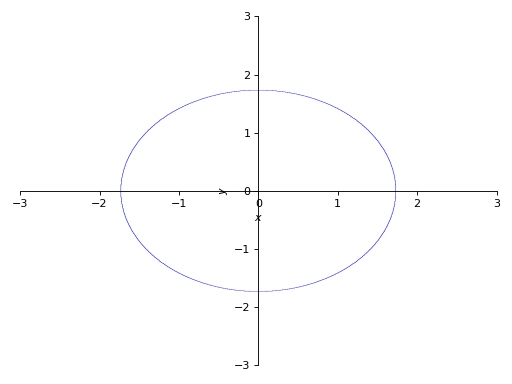
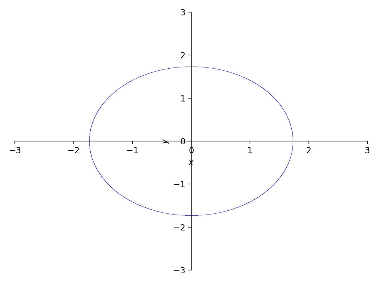
With the range for the symbols:

>>> p2 = plot_implicit(
...     Eq(x**2 + y**2, 3), (x, -3, 3), (y, -3, 3))

(png, hires.png, pdf)

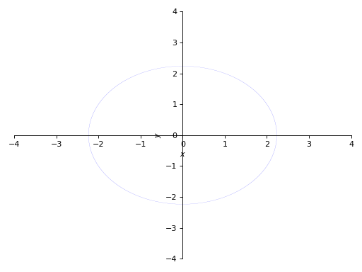
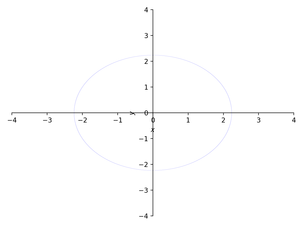
With depth of recursion as argument:

>>> p3 = plot_implicit(
...     Eq(x**2 + y**2, 5), (x, -4, 4), (y, -4, 4), depth = 2)

(png, hires.png, pdf)

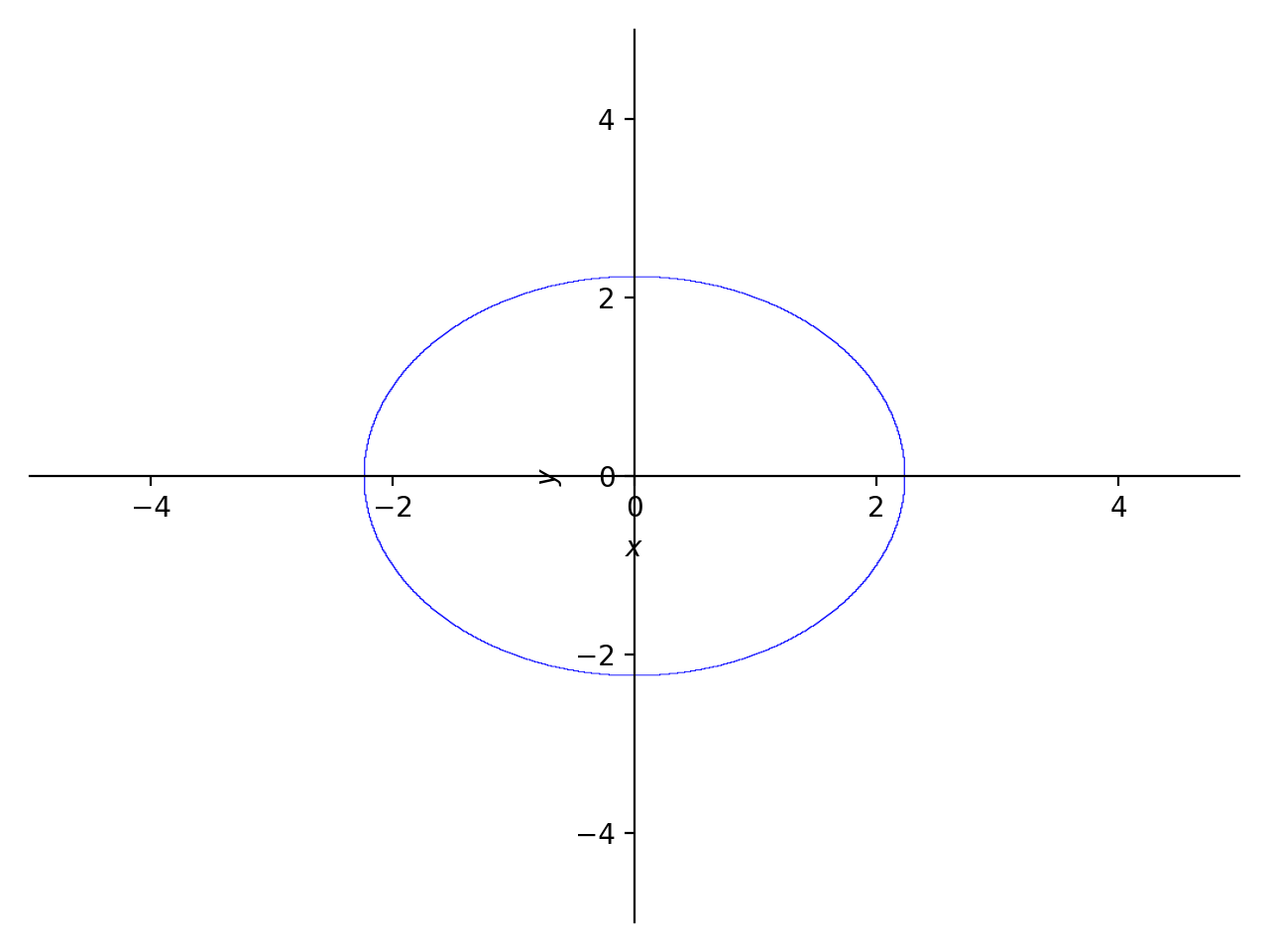
Using mesh grid and not using adaptive meshing:

>>> p4 = plot_implicit(
...     Eq(x**2 + y**2, 5), (x, -5, 5), (y, -2, 2),
...     adaptive=False)

(png, hires.png, pdf)

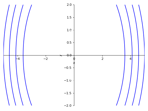
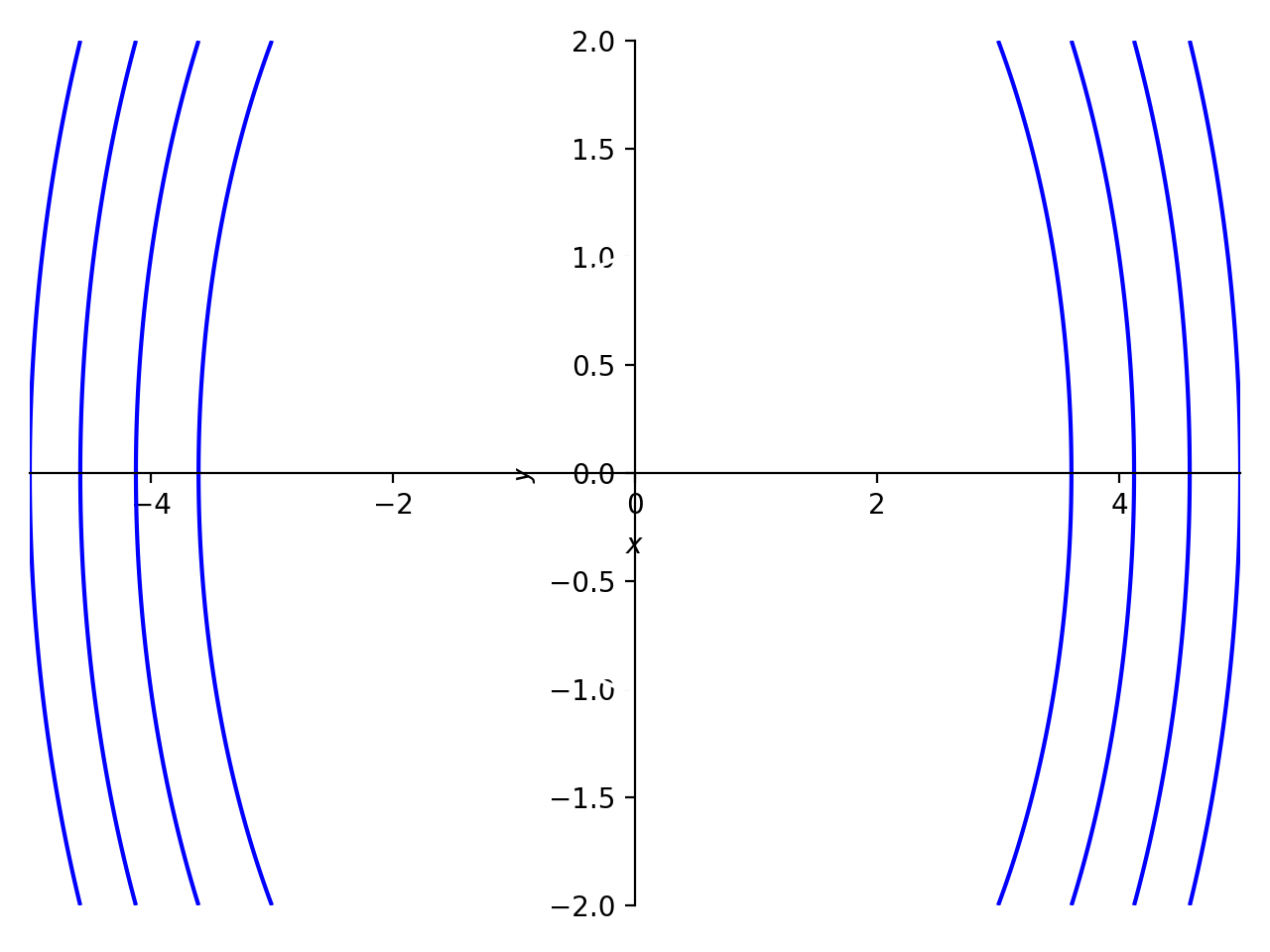
Using mesh grid without using adaptive meshing with number of points specified:

>>> p5 = plot_implicit(
...     Eq(x**2 + y**2, 5), (x, -5, 5), (y, -2, 2),
...     adaptive=False, n=400)

(png, hires.png, pdf)

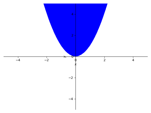
Plotting regions:

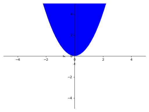
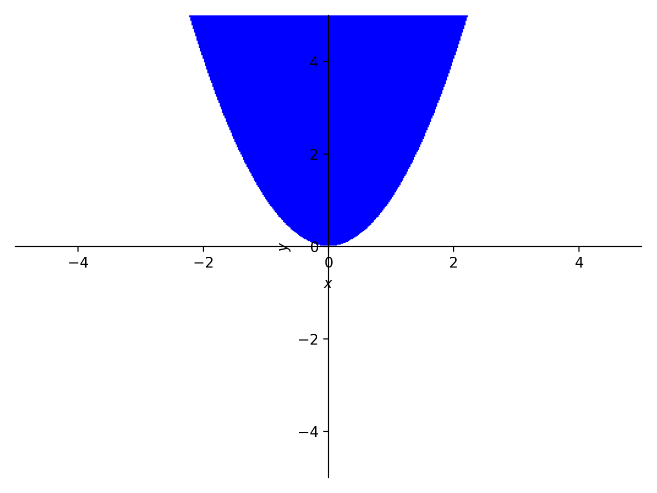
>>> p6 = plot_implicit(y > x**2)

(png, hires.png, pdf)

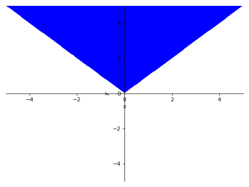
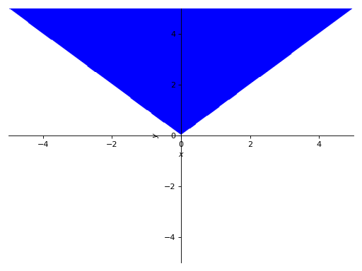
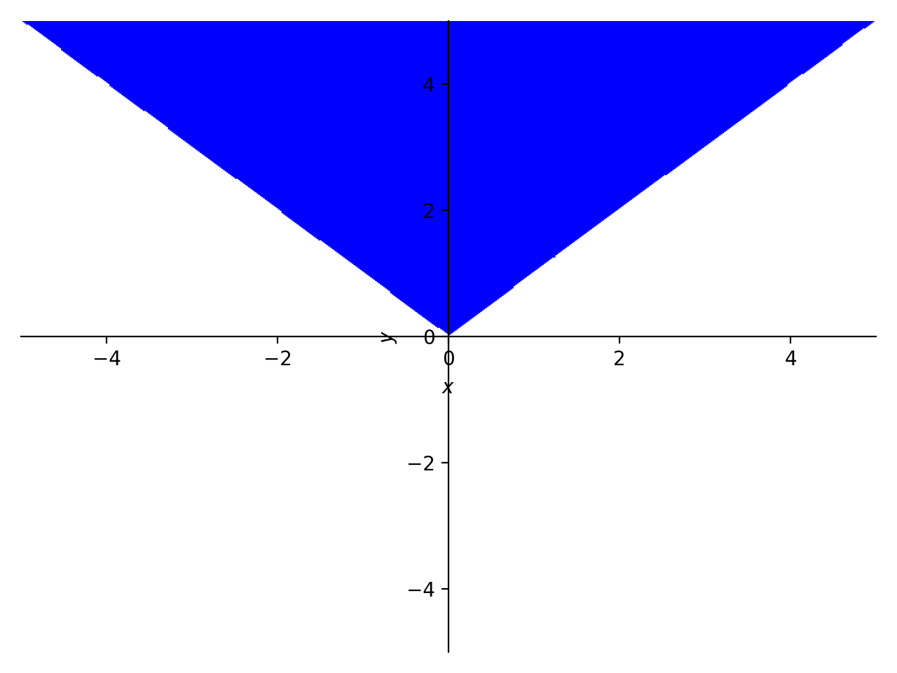
Plotting Using boolean conjunctions:

>>> p7 = plot_implicit(And(y > x, y > -x))

(png, hires.png, pdf)

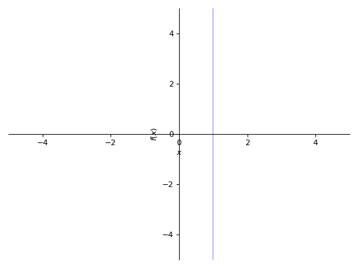
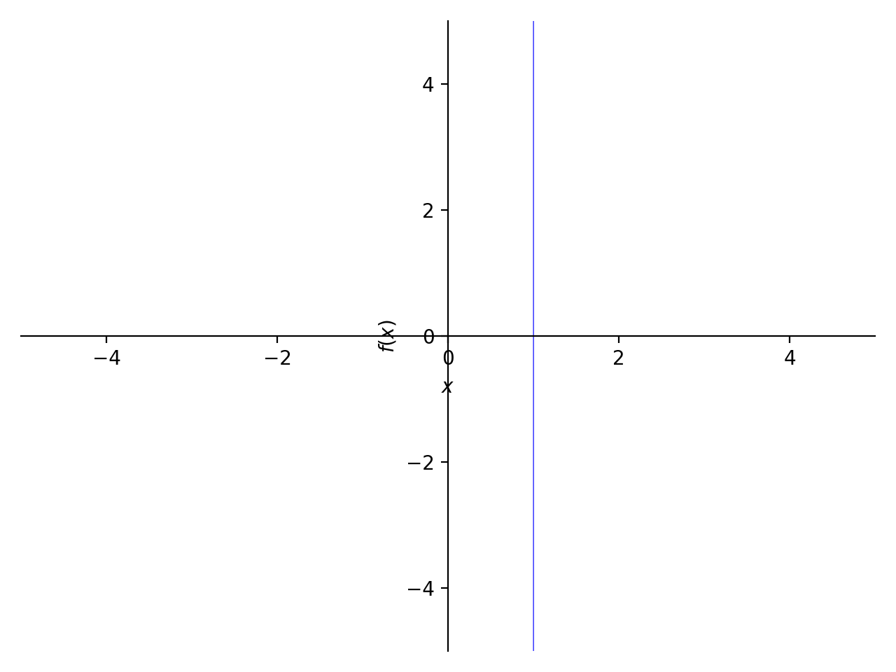
When plotting an expression with a single variable (y - 1, for example), specify the x or the y variable explicitly:

>>> p8 = plot_implicit(y - 1, y_var=y)
>>> p9 = plot_implicit(x - 1, x_var=x)

(png, hires.png, pdf)

(png, hires.png, pdf)

PlotGrid Class

class sympy.plotting.plot.PlotGrid(

nrows,

ncolumns,

*args,

show=True,

size=None,

**kwargs,

)

This class helps to plot subplots from already created SymPy plots in a single figure.

Examples

>>> from sympy import symbols
>>> from sympy.plotting import plot, plot3d, PlotGrid
>>> x, y = symbols('x, y')
>>> p1 = plot(x, x**2, x**3, (x, -5, 5))
>>> p2 = plot((x**2, (x, -6, 6)), (x, (x, -5, 5)))
>>> p3 = plot(x**3, (x, -5, 5))
>>> p4 = plot3d(x*y, (x, -5, 5), (y, -5, 5))

(png, hires.png, pdf)

(png, hires.png, pdf)

(png, hires.png, pdf)

(png, hires.png, pdf)

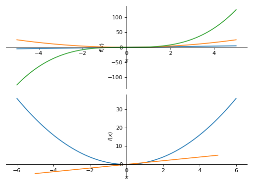
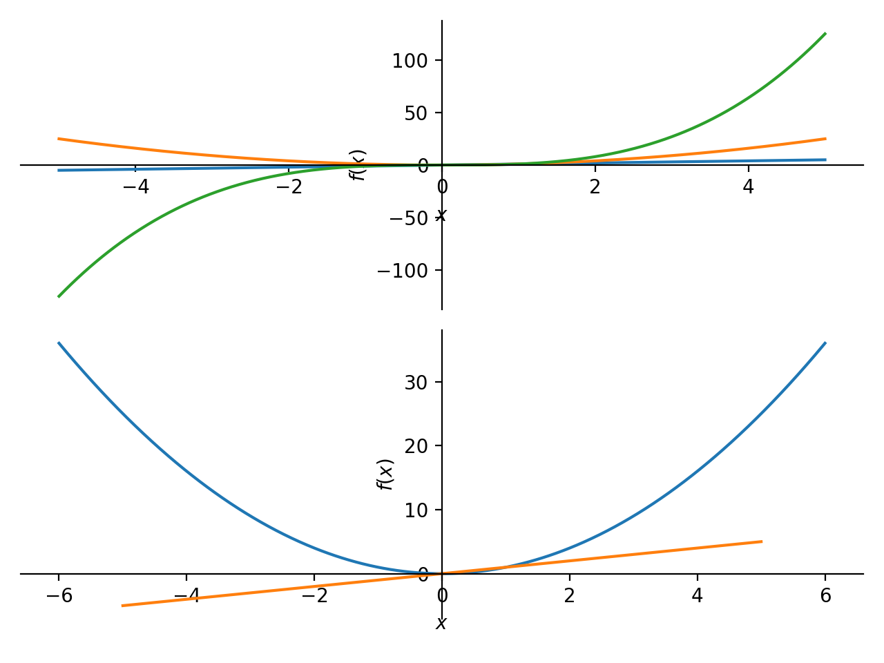
Plotting vertically in a single line:

>>> PlotGrid(2, 1, p1, p2)
PlotGrid object containing:
Plot[0]:Plot object containing:
[0]: cartesian line: x for x over (-5.0, 5.0)
[1]: cartesian line: x**2 for x over (-5.0, 5.0)
[2]: cartesian line: x**3 for x over (-5.0, 5.0)
Plot[1]:Plot object containing:
[0]: cartesian line: x**2 for x over (-6.0, 6.0)
[1]: cartesian line: x for x over (-5.0, 5.0)

(png, hires.png, pdf)

Plotting horizontally in a single line:

>>> PlotGrid(1, 3, p2, p3, p4)
PlotGrid object containing:
Plot[0]:Plot object containing:
[0]: cartesian line: x**2 for x over (-6.0, 6.0)
[1]: cartesian line: x for x over (-5.0, 5.0)
Plot[1]:Plot object containing:
[0]: cartesian line: x**3 for x over (-5.0, 5.0)
Plot[2]:Plot object containing:
[0]: cartesian surface: x*y for x over (-5.0, 5.0) and y over (-5.0, 5.0)

(png, hires.png, pdf)

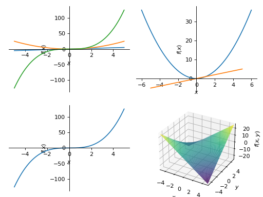
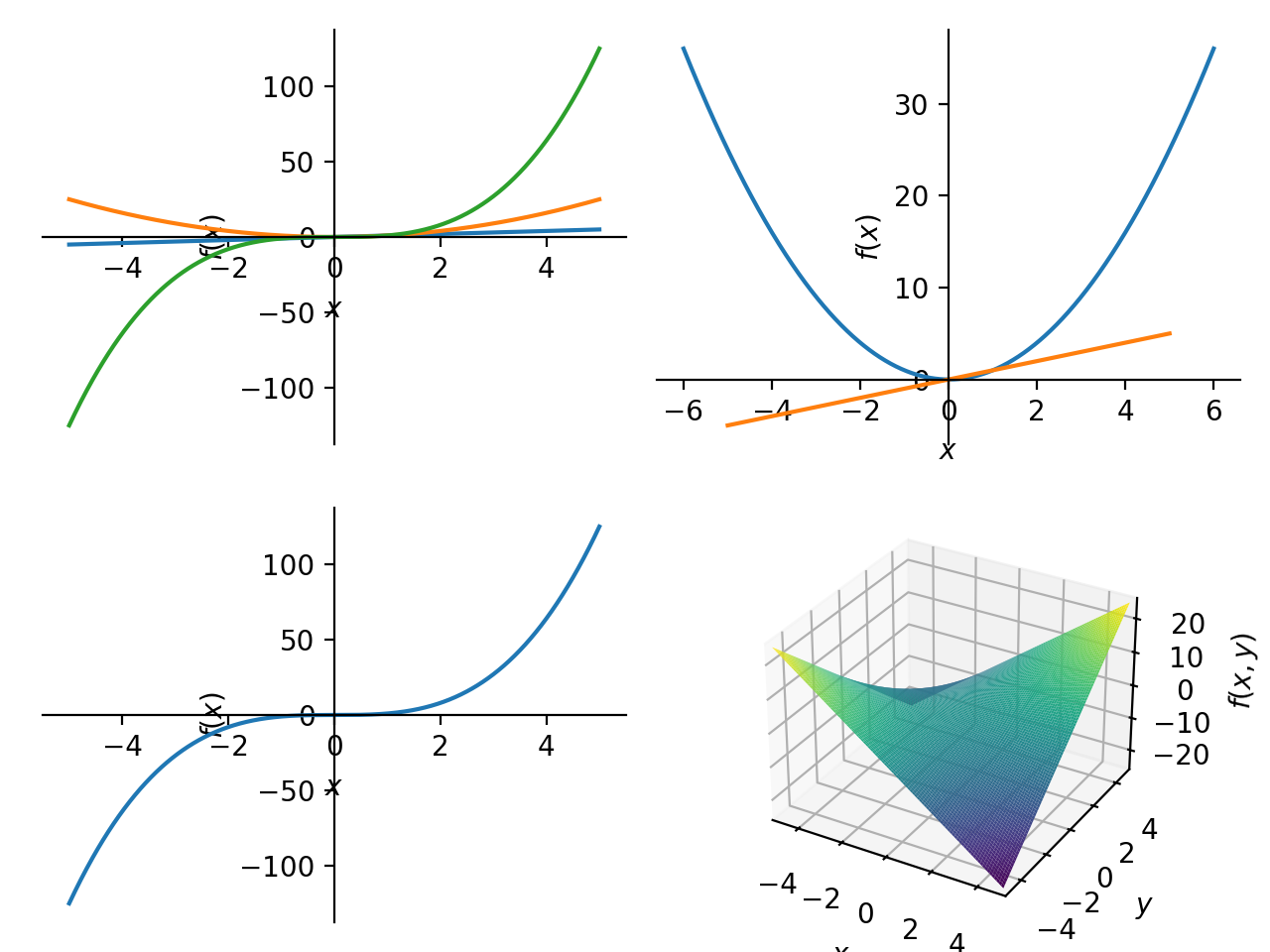
Plotting in a grid form:

>>> PlotGrid(2, 2, p1, p2, p3, p4)
PlotGrid object containing:
Plot[0]:Plot object containing:
[0]: cartesian line: x for x over (-5.0, 5.0)
[1]: cartesian line: x**2 for x over (-5.0, 5.0)
[2]: cartesian line: x**3 for x over (-5.0, 5.0)
Plot[1]:Plot object containing:
[0]: cartesian line: x**2 for x over (-6.0, 6.0)
[1]: cartesian line: x for x over (-5.0, 5.0)
Plot[2]:Plot object containing:
[0]: cartesian line: x**3 for x over (-5.0, 5.0)
Plot[3]:Plot object containing:
[0]: cartesian surface: x*y for x over (-5.0, 5.0) and y over (-5.0, 5.0)

(png, hires.png, pdf)

Series Classes

class sympy.plotting.series.BaseSeries(*args, **kwargs)

Base class for the data objects containing stuff to be plotted.

Notes

The backend should check if it supports the data series that is given. (e.g. TextBackend supports only LineOver1DRangeSeries). It is the backend responsibility to know how to use the class of data series that is given.

Some data series classes are grouped (using a class attribute like is_2Dline) according to the api they present (based only on convention). The backend is not obliged to use that api (e.g. LineOver1DRangeSeries belongs to the is_2Dline group and presents the get_points method, but the TextBackend does not use the get_points method).

BaseSeries

eval_color_func(*args)

Evaluate the color function.

Parameters:

args : tuple

Arguments to be passed to the coloring function. Can be coordinates or parameters or both.

Notes

The backend will request the data series to generate the numerical data. Depending on the data series, either the data series itself or the backend will eventually execute this function to generate the appropriate coloring value.

property expr

Return the expression (or expressions) of the series.

get_data()

Compute and returns the numerical data.

The number of parameters returned by this method depends on the specific instance. If s is the series, make sure to read help(s.get_data) to understand what it returns.

get_label(

use_latex=False,

wrapper='$%s$',

)

Return the label to be used to display the expression.

Parameters:

use_latex : bool

If False, the string representation of the expression is returned. If True, the latex representation is returned.

wrapper : str

The backend might need the latex representation to be wrapped by some characters. Default to "$%s$".

Returns:

label : str

property n

Returns a list [n1, n2, n3] of numbers of discratization points.

property params

Get or set the current parameters dictionary.

Parameters:

p : dict

• key: symbol associated to the parameter

• val: the numeric value

class sympy.plotting.series.Line2DBaseSeries(**kwargs)

A base class for 2D lines.

• adding the label, steps and only_integers options

• making is_2Dline true

• defining get_segments and get_color_array

get_data()

Return coordinates for plotting the line.

Returns:

x: np.ndarray

x-coordinates

y: np.ndarray

y-coordinates

z: np.ndarray (optional)

z-coordinates in case of Parametric3DLineSeries, Parametric3DLineInteractiveSeries

param : np.ndarray (optional)

The parameter in case of Parametric2DLineSeries, Parametric3DLineSeries or AbsArgLineSeries (and their corresponding interactive series).

class sympy.plotting.series.LineOver1DRangeSeries(

expr,

var_start_end,

label='',

**kwargs,

)

Representation for a line consisting of a SymPy expression over a range.

get_points()

Return lists of coordinates for plotting. Depending on the adaptive option, this function will either use an adaptive algorithm or it will uniformly sample the expression over the provided range.

This function is available for back-compatibility purposes. Consider using get_data() instead.

Returns:

x : list

List of x-coordinates

ylist

List of y-coordinates

class sympy.plotting.series.Parametric2DLineSeries(

expr_x,

expr_y,

var_start_end,

label='',

**kwargs,

)

Representation for a line consisting of two parametric SymPy expressions over a range.

class sympy.plotting.series.Line3DBaseSeries

A base class for 3D lines.

Most of the stuff is derived from Line2DBaseSeries.

class sympy.plotting.series.Parametric3DLineSeries(

expr_x,

expr_y,

expr_z,

var_start_end,

label='',

**kwargs,

)

Representation for a 3D line consisting of three parametric SymPy expressions and a range.

class sympy.plotting.series.SurfaceBaseSeries(*args, **kwargs)

A base class for 3D surfaces.

class sympy.plotting.series.SurfaceOver2DRangeSeries(

expr,

var_start_end_x,

var_start_end_y,

label='',

**kwargs,

)

Representation for a 3D surface consisting of a SymPy expression and 2D range.

get_data()

Return arrays of coordinates for plotting.

Returns:

mesh_x : np.ndarray

Discretized x-domain.

mesh_y : np.ndarray

Discretized y-domain.

mesh_z : np.ndarray

Results of the evaluation.

get_meshes()

Return the x,y,z coordinates for plotting the surface. This function is available for back-compatibility purposes. Consider using get_data() instead.

class sympy.plotting.series.ParametricSurfaceSeries(

expr_x,

expr_y,

expr_z,

var_start_end_u,

var_start_end_v,

label='',

**kwargs,

)

Representation for a 3D surface consisting of three parametric SymPy expressions and a range.

get_data()

Return arrays of coordinates for plotting.

Returns:

x : np.ndarray [n2 x n1]

x-coordinates.

y : np.ndarray [n2 x n1]

y-coordinates.

z : np.ndarray [n2 x n1]

z-coordinates.

mesh_u : np.ndarray [n2 x n1]

Discretized u range.

mesh_v : np.ndarray [n2 x n1]

Discretized v range.

get_meshes()

Return the x,y,z coordinates for plotting the surface. This function is available for back-compatibility purposes. Consider using get_data() instead.

class sympy.plotting.series.GenericDataSeries(tp, *args, **kwargs)

Represents generic numerical data.

Notes

This class serves the purpose of back-compatibility with the “markers, annotations, fill, rectangles” keyword arguments that represent user-provided numerical data. In particular, it solves the problem of combining together two or more plot-objects with the extend or append methods: user-provided numerical data is also taken into consideration because it is stored in this series class.

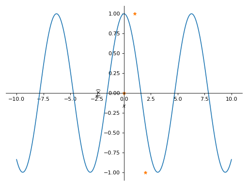
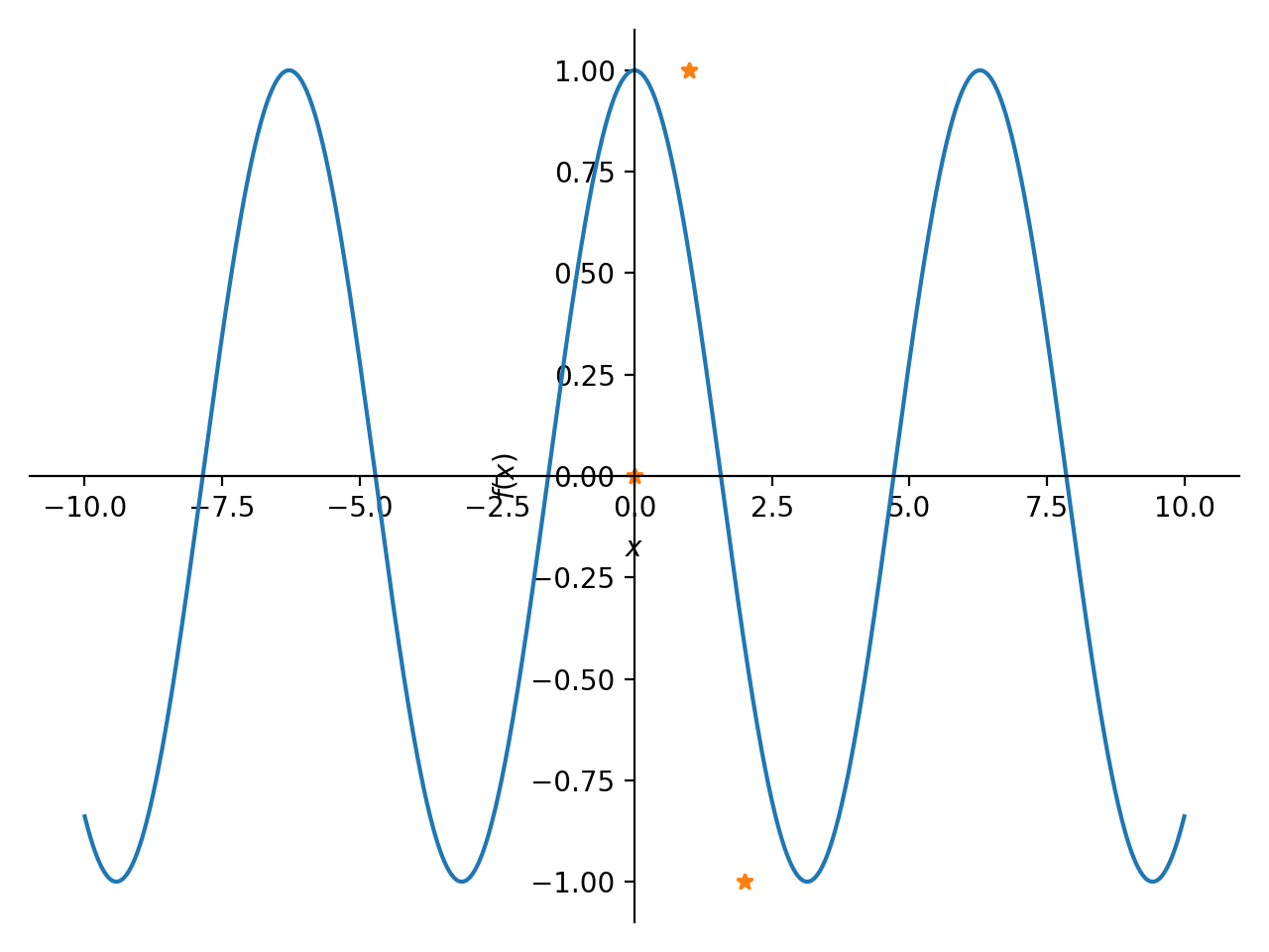
Also note that the current implementation is far from optimal, as each keyword argument is stored into an attribute in the Plot class, which requires a hard-coded if-statement in the MatplotlibBackend class. The implementation suggests that it is ok to add attributes and if-statements to provide more and more functionalities for user-provided numerical data (e.g. adding horizontal lines, or vertical lines, or bar plots, etc). However, in doing so one would reinvent the wheel: plotting libraries (like Matplotlib) already implements the necessary API.

Instead of adding more keyword arguments and attributes, users interested in adding custom numerical data to a plot should retrieve the figure created by this plotting module. For example, this code:

from sympy import Symbol, plot, cos
x = Symbol("x")
p = plot(cos(x), markers=[{"args": [[0, 1, 2], [0, 1, -1], "*"]}])

(png, hires.png, pdf)

Becomes:

p = plot(cos(x), backend="matplotlib")
fig, ax = p._backend.fig, p._backend.ax
ax.plot([0, 1, 2], [0, 1, -1], "*")
fig

(png, hires.png, pdf)

Which is far better in terms of readibility. Also, it gives access to the full plotting library capabilities, without the need to reinvent the wheel.

class sympy.plotting.series.ImplicitSeries(

expr,

var_start_end_x,

var_start_end_y,

label='',

**kwargs,

)

Representation for 2D Implicit plot.

get_data()

Returns numerical data.

Returns:

If the series is evaluated with the \(adaptive=True\) it returns:

interval_list : list

List of bounding rectangular intervals to be postprocessed and eventually used with Matplotlib’s fill command.

dummy : str

A string containing "fill".

Otherwise, it returns 2D numpy arrays to be used with Matplotlib’s

contour or contourf commands:

x_array : np.ndarray

y_array : np.ndarray

z_array : np.ndarray

plot_type : str

A string specifying which plot command to use, "contour" or "contourf".

get_label(

use_latex=False,

wrapper='$%s$',

)

Return the label to be used to display the expression.

Parameters:

use_latex : bool

If False, the string representation of the expression is returned. If True, the latex representation is returned.

wrapper : str

The backend might need the latex representation to be wrapped by some characters. Default to "$%s$".

Returns:

label : str

Backends

class sympy.plotting.plot.MatplotlibBackend(*series, **kwargs)

This class implements the functionalities to use Matplotlib with SymPy plotting functions.

static get_segments(x, y, z=None)

Convert two list of coordinates to a list of segments to be used with Matplotlib’s LineCollection.

Parameters:

x : list

List of x-coordinates

ylist

List of y-coordinates

zlist

List of z-coordinates for a 3D line.

process_series()

Iterates over every Plot object and further calls _process_series()

class sympy.plotting.plot.TextBackend(*args, **kwargs)

Pyglet Plotting

This is the documentation for the old plotting module that uses pyglet. This module has some limitations and is not actively developed anymore. For an alternative you can look at the new plotting module.

The pyglet plotting module can do nice 2D and 3D plots that can be controlled by console commands as well as keyboard and mouse, with the only dependency being pyglet.

Here is the simplest usage:

>>> from sympy import var
>>> from sympy.plotting.pygletplot import PygletPlot as Plot
>>> var('x y z')
>>> Plot(x*y**3-y*x**3)

To see lots of plotting examples, see examples/pyglet_plotting.py and try running it in interactive mode (python -i plotting.py):

$ python -i examples/pyglet_plotting.py

And type for instance example(7) or example(11).

See also the Plotting Module wiki page for screenshots.

Plot Window Controls

Camera	Keys
Sensitivity Modifier	SHIFT
Zoom	R and F, Page Up and Down, Numpad + and -
Rotate View X,Y axis	Arrow Keys, A,S,D,W, Numpad 4,6,8,2
Rotate View Z axis	Q and E, Numpad 7 and 9
Rotate Ordinate Z axis	Z and C, Numpad 1 and 3
View XY	F1
View XZ	F2
View YZ	F3
View Perspective	F4
Reset	X, Numpad 5

Axes	Keys
Toggle Visible	F5
Toggle Colors	F6

Window	Keys
Close	ESCAPE
Screenshot	F8

The mouse can be used to rotate, zoom, and translate by dragging the left, middle, and right mouse buttons respectively.

Coordinate Modes

Plot supports several curvilinear coordinate modes, and they are independent for each plotted function. You can specify a coordinate mode explicitly with the ‘mode’ named argument, but it can be automatically determined for cartesian or parametric plots, and therefore must only be specified for polar, cylindrical, and spherical modes.

Specifically, Plot(function arguments) and Plot.__setitem__(i, function arguments) (accessed using array-index syntax on the Plot instance) will interpret your arguments as a cartesian plot if you provide one function and a parametric plot if you provide two or three functions. Similarly, the arguments will be interpreted as a curve is one variable is used, and a surface if two are used.

Supported mode names by number of variables:

• 1 (curves): parametric, cartesian, polar

• 2 (surfaces): parametric, cartesian, cylindrical, spherical

>>> Plot(1, 'mode=spherical; color=zfade4')

Note that function parameters are given as option strings of the form "key1=value1; key2 = value2" (spaces are truncated). Keyword arguments given directly to plot apply to the plot itself.

Specifying Intervals for Variables

The basic format for variable intervals is [var, min, max, steps]. However, the syntax is quite flexible, and arguments not specified are taken from the defaults for the current coordinate mode:

>>> Plot(x**2) # implies [x,-5,5,100]
>>> Plot(x**2, [], []) # [x,-1,1,40], [y,-1,1,40]
>>> Plot(x**2-y**2, [100], [100]) # [x,-1,1,100], [y,-1,1,100]
>>> Plot(x**2, [x,-13,13,100])
>>> Plot(x**2, [-13,13]) # [x,-13,13,100]
>>> Plot(x**2, [x,-13,13]) # [x,-13,13,100]
>>> Plot(1*x, [], [x], 'mode=cylindrical') # [unbound_theta,0,2*Pi,40], [x,-1,1,20]

Using the Interactive Interface

>>> p = Plot(visible=False)
>>> f = x**2
>>> p[1] = f
>>> p[2] = f.diff(x)
>>> p[3] = f.diff(x).diff(x)
>>> p
[1]: x**2, 'mode=cartesian'
[2]: 2*x, 'mode=cartesian'
[3]: 2, 'mode=cartesian'
>>> p.show()
>>> p.clear()
>>> p
<blank plot>
>>> p[1] =  x**2+y**2
>>> p[1].style = 'solid'
>>> p[2] = -x**2-y**2
>>> p[2].style = 'wireframe'
>>> p[1].color = z, (0.4,0.4,0.9), (0.9,0.4,0.4)
>>> p[1].style = 'both'
>>> p[2].style = 'both'
>>> p.close()

Using Custom Color Functions

The following code plots a saddle and color it by the magnitude of its gradient:

>>> fz = x**2-y**2
>>> Fx, Fy, Fz = fz.diff(x), fz.diff(y), 0
>>> p[1] = fz, 'style=solid'
>>> p[1].color = (Fx**2 + Fy**2 + Fz**2)**(0.5)

The coloring algorithm works like this:

1. Evaluate the color function(s) across the curve or surface.

2. Find the minimum and maximum value of each component.

3. Scale each component to the color gradient.

When not specified explicitly, the default color gradient is \(f(0.0)=(0.4,0.4,0.4) \rightarrow f(1.0)=(0.9,0.9,0.9)\). In our case, everything is gray-scale because we have applied the default color gradient uniformly for each color component. When defining a color scheme in this way, you might want to supply a color gradient as well:

>>> p[1].color = (Fx**2 + Fy**2 + Fz**2)**(0.5), (0.1,0.1,0.9), (0.9,0.1,0.1)

Here’s a color gradient with four steps:

>>> gradient = [ 0.0, (0.1,0.1,0.9), 0.3, (0.1,0.9,0.1),
...              0.7, (0.9,0.9,0.1), 1.0, (1.0,0.0,0.0) ]
>>> p[1].color = (Fx**2 + Fy**2 + Fz**2)**(0.5), gradient

The other way to specify a color scheme is to give a separate function for each component r, g, b. With this syntax, the default color scheme is defined:

>>> p[1].color = z,y,x, (0.4,0.4,0.4), (0.9,0.9,0.9)

This maps z->red, y->green, and x->blue. In some cases, you might prefer to use the following alternative syntax:

>>> p[1].color = z,(0.4,0.9), y,(0.4,0.9), x,(0.4,0.9)

You can still use multi-step gradients with three-function color schemes.

Plotting Geometric Entities

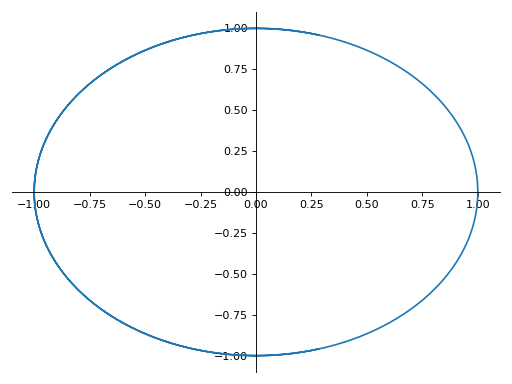
The plotting module is capable of plotting some 2D geometric entities like line, circle and ellipse. The following example plots a circle centred at origin and of radius 2 units.

>>> from sympy import *
>>> x,y = symbols('x y')
>>> plot_implicit(Eq(x**2+y**2, 4))

Similarly, plot_implicit() may be used to plot any 2-D geometric structure from its implicit equation.

Plotting polygons (Polygon, RegularPolygon, Triangle) are not supported directly.

Plotting with ASCII art

sympy.plotting.textplot.textplot(expr, a, b, W=55, H=21)

Print a crude ASCII art plot of the SymPy expression ‘expr’ (which should contain a single symbol, e.g. x or something else) over the interval [a, b].

Examples

>>> from sympy import Symbol, sin
>>> from sympy.plotting import textplot
>>> t = Symbol('t')
>>> textplot(sin(t)*t, 0, 15)
 14 |                                                  ...
    |                                                     .
    |                                                 .
    |                                                      .
    |                                                .
    |                            ...
    |                           /   .               .
    |                          /
    |                         /      .
    |                        .        .            .
1.5 |----.......--------------------------------------------
    |....       \           .          .
    |            \         /                      .
    |             ..      /             .
    |               \    /                       .
    |                ....
    |                                    .
    |                                     .     .
    |
    |                                      .   .
-11 |_______________________________________________________
     0                          7.5                        15