Control System Plots

This module contains plotting functions for some of the common plots used in control system. Matplotlib will be required as an external dependency if the user wants the plots. To get only the numerical data of the plots, NumPy will be required as external dependency.

Pole-Zero Plot

control_plots.pole_zero_plot(

pole_color='blue',

pole_markersize=10,

zero_color='orange',

zero_markersize=7,

grid=True,

show_axes=True,

show=True,

**kwargs,

)

Returns the Pole-Zero plot (also known as PZ Plot or PZ Map) of a system.

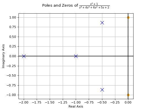
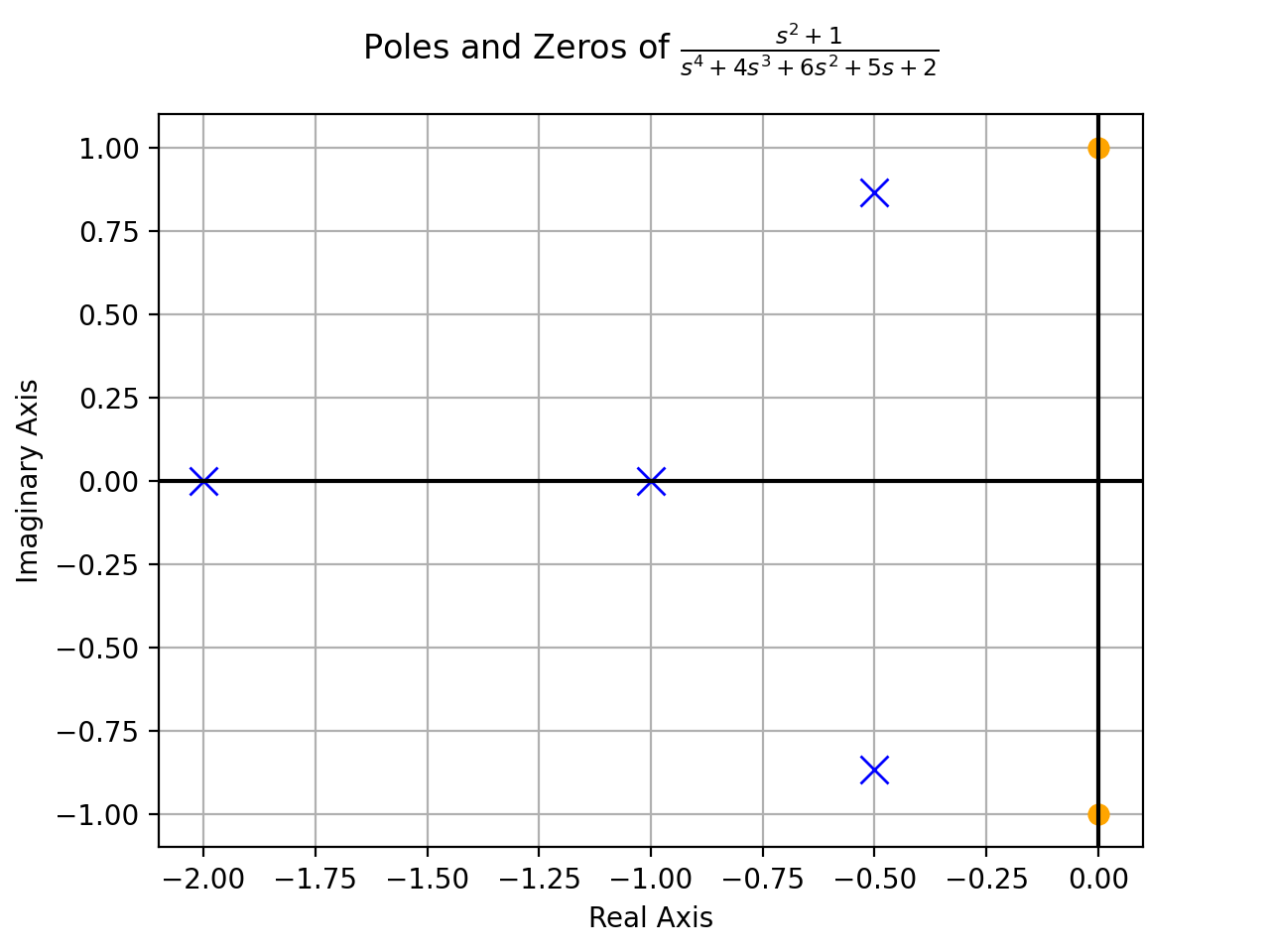
A Pole-Zero plot is a graphical representation of a system’s poles and zeros. It is plotted on a complex plane, with circular markers representing the system’s zeros and ‘x’ shaped markers representing the system’s poles.

Parameters:

system : SISOLinearTimeInvariant type systems

The system for which the pole-zero plot is to be computed.

pole_color : str, tuple, optional

The color of the pole points on the plot. Default color is blue. The color can be provided as a matplotlib color string, or a 3-tuple of floats each in the 0-1 range.

pole_markersize : Number, optional

The size of the markers used to mark the poles in the plot. Default pole markersize is 10.

zero_color : str, tuple, optional

The color of the zero points on the plot. Default color is orange. The color can be provided as a matplotlib color string, or a 3-tuple of floats each in the 0-1 range.

zero_markersize : Number, optional

The size of the markers used to mark the zeros in the plot. Default zero markersize is 7.

grid : boolean, optional

If True, the plot will have a grid. Defaults to True.

show_axes : boolean, optional

If True, the coordinate axes will be shown. Defaults to False.

show : boolean, optional

If True, the plot will be displayed otherwise the equivalent matplotlib plot object will be returned. Defaults to True.

Examples

>>> from sympy.abc import s
>>> from sympy.physics.control.lti import TransferFunction
>>> from sympy.physics.control.control_plots import pole_zero_plot
>>> tf1 = TransferFunction(s**2 + 1, s**4 + 4*s**3 + 6*s**2 + 5*s + 2, s)
>>> pole_zero_plot(tf1)   

(png, hires.png, pdf)

See also

pole_zero_numerical_data

References

[R730]

https://en.wikipedia.org/wiki/Pole%E2%80%93zero_plot

control_plots.pole_zero_numerical_data()

Returns the numerical data of poles and zeros of the system. It is internally used by pole_zero_plot to get the data for plotting poles and zeros. Users can use this data to further analyse the dynamics of the system or plot using a different backend/plotting-module.

Parameters:

system : SISOLinearTimeInvariant

The system for which the pole-zero data is to be computed.

Returns:

tuple : (zeros, poles)

zeros = Zeros of the system as a list of Python float/complex. poles = Poles of the system as a list of Python float/complex.

Raises:

NotImplementedError

When a SISO LTI system is not passed.

When time delay terms are present in the system.

ValueError

When more than one free symbol is present in the system. The only variable in the transfer function should be the variable of the Laplace transform.

Examples

>>> from sympy.abc import s
>>> from sympy.physics.control.lti import TransferFunction
>>> from sympy.physics.control.control_plots import pole_zero_numerical_data
>>> tf1 = TransferFunction(s**2 + 1, s**4 + 4*s**3 + 6*s**2 + 5*s + 2, s)
>>> pole_zero_numerical_data(tf1)
([-1j, 1j], [-2.0, -1.0, (-0.5-0.8660254037844386j), (-0.5+0.8660254037844386j)])

See also

pole_zero_plot

Bode Plot

control_plots.bode_plot(

initial_exp=-5,

final_exp=5,

grid=True,

show_axes=False,

show=True,

freq_unit='rad/sec',

phase_unit='rad',

phase_unwrap=True,

**kwargs,

)

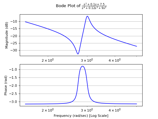
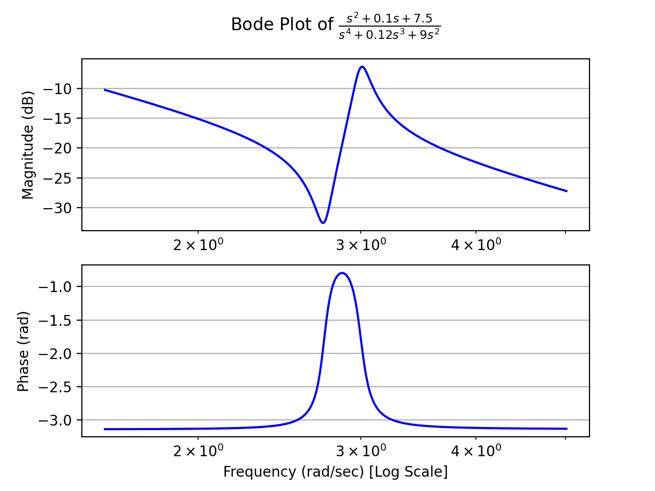
Returns the Bode phase and magnitude plots of a continuous-time system.

Parameters:

system : SISOLinearTimeInvariant type

The LTI SISO system for which the Bode Plot is to be computed.

initial_exp : Number, optional

The initial exponent of 10 of the semilog plot. Defaults to -5.

final_exp : Number, optional

The final exponent of 10 of the semilog plot. Defaults to 5.

show : boolean, optional

If True, the plot will be displayed otherwise the equivalent matplotlib plot object will be returned. Defaults to True.

prec : int, optional

The decimal point precision for the point coordinate values. Defaults to 8.

grid : boolean, optional

If True, the plot will have a grid. Defaults to True.

show_axes : boolean, optional

If True, the coordinate axes will be shown. Defaults to False.

freq_unit : string, optional

User can choose between 'rad/sec' (radians/second) and 'Hz' (Hertz) as frequency units.

phase_unit : string, optional

User can choose between 'rad' (radians) and 'deg' (degree) as phase units.

Examples

>>> from sympy.abc import s
>>> from sympy.physics.control.lti import TransferFunction
>>> from sympy.physics.control.control_plots import bode_plot
>>> tf1 = TransferFunction(1*s**2 + 0.1*s + 7.5, 1*s**4 + 0.12*s**3 + 9*s**2, s)
>>> bode_plot(tf1, initial_exp=0.2, final_exp=0.7)   

(png, hires.png, pdf)

See also

bode_magnitude_plot, bode_phase_plot

control_plots.bode_magnitude_plot(

initial_exp=-5,

final_exp=5,

color='b',

show_axes=False,

grid=True,

show=True,

freq_unit='rad/sec',

**kwargs,

)

Returns the Bode magnitude plot of a continuous-time system.

See bode_plot for all the parameters.

control_plots.bode_phase_plot(

initial_exp=-5,

final_exp=5,

color='b',

show_axes=False,

grid=True,

show=True,

freq_unit='rad/sec',

phase_unit='rad',

phase_unwrap=True,

**kwargs,

)

Returns the Bode phase plot of a continuous-time system.

See bode_plot for all the parameters.

control_plots.bode_magnitude_numerical_data(

initial_exp=-5,

final_exp=5,

freq_unit='rad/sec',

**kwargs,

)

Returns the numerical data of the Bode magnitude plot of the system. It is internally used by bode_magnitude_plot to get the data for plotting Bode magnitude plot. Users can use this data to further analyse the dynamics of the system or plot using a different backend/plotting-module.

Parameters:

system : SISOLinearTimeInvariant

The system for which the data is to be computed.

initial_exp : Number, optional

The initial exponent of 10 of the semilog plot. Defaults to -5.

final_exp : Number, optional

The final exponent of 10 of the semilog plot. Defaults to 5.

freq_unit : string, optional

User can choose between 'rad/sec' (radians/second) and 'Hz' (Hertz) as frequency units.

Returns:

tuple : (x, y)

x = x-axis values of the Bode magnitude plot. y = y-axis values of the Bode magnitude plot.

Raises:

NotImplementedError

When a SISO LTI system is not passed.

When time delay terms are present in the system.

ValueError

When more than one free symbol is present in the system. The only variable in the transfer function should be the variable of the Laplace transform.

When incorrect frequency units are given as input.

Examples

>>> from sympy.abc import s
>>> from sympy.physics.control.lti import TransferFunction
>>> from sympy.physics.control.control_plots import bode_magnitude_numerical_data
>>> tf1 = TransferFunction(s**2 + 1, s**4 + 4*s**3 + 6*s**2 + 5*s + 2, s)
>>> bode_magnitude_numerical_data(tf1)   
([1e-05, 1.5148378120533502e-05,..., 68437.36188804005, 100000.0],
[-6.020599914256786, -6.0205999155219505,..., -193.4117304087953, -200.00000000260573])

See also

bode_magnitude_plot, bode_phase_numerical_data

control_plots.bode_phase_numerical_data(

initial_exp=-5,

final_exp=5,

freq_unit='rad/sec',

phase_unit='rad',

phase_unwrap=True,

**kwargs,

)

Returns the numerical data of the Bode phase plot of the system. It is internally used by bode_phase_plot to get the data for plotting Bode phase plot. Users can use this data to further analyse the dynamics of the system or plot using a different backend/plotting-module.

Parameters:

system : SISOLinearTimeInvariant

The system for which the Bode phase plot data is to be computed.

initial_exp : Number, optional

The initial exponent of 10 of the semilog plot. Defaults to -5.

final_exp : Number, optional

The final exponent of 10 of the semilog plot. Defaults to 5.

freq_unit : string, optional

User can choose between 'rad/sec' (radians/second) and ‘``’Hz’`` (Hertz) as frequency units.

phase_unit : string, optional

User can choose between 'rad' (radians) and 'deg' (degree) as phase units.

phase_unwrap : bool, optional

Set to True by default.

Returns:

tuple : (x, y)

x = x-axis values of the Bode phase plot. y = y-axis values of the Bode phase plot.

Raises:

NotImplementedError

When a SISO LTI system is not passed.

When time delay terms are present in the system.

ValueError

When more than one free symbol is present in the system. The only variable in the transfer function should be the variable of the Laplace transform.

When incorrect frequency or phase units are given as input.

Examples

>>> from sympy.abc import s
>>> from sympy.physics.control.lti import TransferFunction
>>> from sympy.physics.control.control_plots import bode_phase_numerical_data
>>> tf1 = TransferFunction(s**2 + 1, s**4 + 4*s**3 + 6*s**2 + 5*s + 2, s)
>>> bode_phase_numerical_data(tf1)   
([1e-05, 1.4472354033813751e-05, 2.035581932165858e-05,..., 47577.3248186011, 67884.09326036123, 100000.0],
[-2.5000000000291665e-05, -3.6180885085e-05, -5.08895483066e-05,...,-3.1415085799262523, -3.14155265358979])

See also

bode_magnitude_plot, bode_phase_numerical_data

Impulse-Response Plot

control_plots.impulse_response_plot(

color='b',

prec=8,

lower_limit=0,

upper_limit=10,

show_axes=False,

grid=True,

show=True,

**kwargs,

)

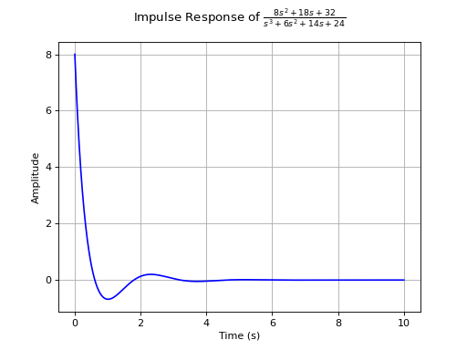
Returns the unit impulse response (Input is the Dirac-Delta Function) of a continuous-time system.

Parameters:

system : SISOLinearTimeInvariant type

The LTI SISO system for which the Impulse Response is to be computed.

color : str, tuple, optional

The color of the line. Default is Blue.

show : boolean, optional

If True, the plot will be displayed otherwise the equivalent matplotlib plot object will be returned. Defaults to True.

lower_limit : Number, optional

The lower limit of the plot range. Defaults to 0.

upper_limit : Number, optional

The upper limit of the plot range. Defaults to 10.

prec : int, optional

The decimal point precision for the point coordinate values. Defaults to 8.

show_axes : boolean, optional

If True, the coordinate axes will be shown. Defaults to False.

grid : boolean, optional

If True, the plot will have a grid. Defaults to True.

Examples

>>> from sympy.abc import s
>>> from sympy.physics.control.lti import TransferFunction
>>> from sympy.physics.control.control_plots import impulse_response_plot
>>> tf1 = TransferFunction(8*s**2 + 18*s + 32, s**3 + 6*s**2 + 14*s + 24, s)
>>> impulse_response_plot(tf1)   

(png, hires.png, pdf)

See also

step_response_plot, ramp_response_plot

References

[R731]

https://www.mathworks.com/help/control/ref/dynamicsystem.impulse.html

control_plots.impulse_response_numerical_data(

prec=8,

lower_limit=0,

upper_limit=10,

**kwargs,

)

Returns the numerical values of the points in the impulse response plot of a SISO continuous-time system. By default, adaptive sampling is used. If the user wants to instead get an uniformly sampled response, then adaptive kwarg should be passed False and n must be passed as additional kwargs. Refer to the parameters of class sympy.plotting.series.LineOver1DRangeSeries for more details.

Parameters:

system : SISOLinearTimeInvariant

The system for which the impulse response data is to be computed.

prec : int, optional

The decimal point precision for the point coordinate values. Defaults to 8.

lower_limit : Number, optional

The lower limit of the plot range. Defaults to 0.

upper_limit : Number, optional

The upper limit of the plot range. Defaults to 10.

kwargs :

Additional keyword arguments are passed to the underlying sympy.plotting.series.LineOver1DRangeSeries class.

Returns:

tuple : (x, y)

x = Time-axis values of the points in the impulse response. NumPy array. y = Amplitude-axis values of the points in the impulse response. NumPy array.

Raises:

NotImplementedError

When a SISO LTI system is not passed.

When time delay terms are present in the system.

ValueError

When more than one free symbol is present in the system. The only variable in the transfer function should be the variable of the Laplace transform.

When lower_limit parameter is less than 0.

Examples

>>> from sympy.abc import s
>>> from sympy.physics.control.lti import TransferFunction
>>> from sympy.physics.control.control_plots import impulse_response_numerical_data
>>> tf1 = TransferFunction(s, s**2 + 5*s + 8, s)
>>> impulse_response_numerical_data(tf1)   
([0.0, 0.06616480200395854,... , 9.854500743565858, 10.0],
[0.9999999799999999, 0.7042848373025861,...,7.170748906965121e-13, -5.1901263495547205e-12])

See also

impulse_response_plot

Step-Response Plot

control_plots.step_response_plot(

color='b',

prec=8,

lower_limit=0,

upper_limit=10,

show_axes=False,

grid=True,

show=True,

**kwargs,

)

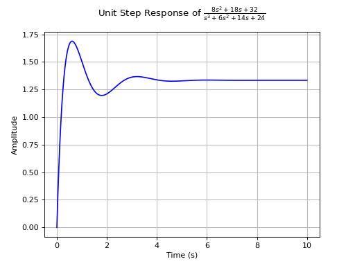
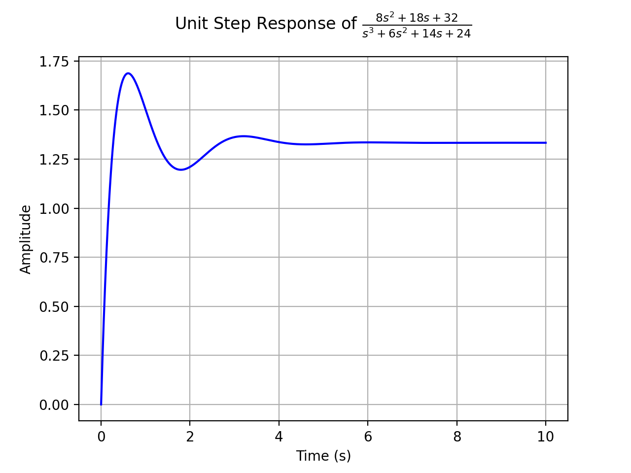
Returns the unit step response of a continuous-time system. It is the response of the system when the input signal is a step function.

Parameters:

system : SISOLinearTimeInvariant type

The LTI SISO system for which the Step Response is to be computed.

color : str, tuple, optional

The color of the line. Default is Blue.

show : boolean, optional

If True, the plot will be displayed otherwise the equivalent matplotlib plot object will be returned. Defaults to True.

lower_limit : Number, optional

The lower limit of the plot range. Defaults to 0.

upper_limit : Number, optional

The upper limit of the plot range. Defaults to 10.

prec : int, optional

The decimal point precision for the point coordinate values. Defaults to 8.

show_axes : boolean, optional

If True, the coordinate axes will be shown. Defaults to False.

grid : boolean, optional

If True, the plot will have a grid. Defaults to True.

Examples

>>> from sympy.abc import s
>>> from sympy.physics.control.lti import TransferFunction
>>> from sympy.physics.control.control_plots import step_response_plot
>>> tf1 = TransferFunction(8*s**2 + 18*s + 32, s**3 + 6*s**2 + 14*s + 24, s)
>>> step_response_plot(tf1)   

(png, hires.png, pdf)

See also

impulse_response_plot, ramp_response_plot

References

[R732]

https://www.mathworks.com/help/control/ref/lti.step.html

control_plots.step_response_numerical_data(

prec=8,

lower_limit=0,

upper_limit=10,

**kwargs,

)

Returns the numerical values of the points in the step response plot of a SISO continuous-time system. By default, adaptive sampling is used. If the user wants to instead get an uniformly sampled response, then adaptive kwarg should be passed False and n must be passed as additional kwargs. Refer to the parameters of class sympy.plotting.series.LineOver1DRangeSeries for more details.

Parameters:

system : SISOLinearTimeInvariant

The system for which the unit step response data is to be computed.

prec : int, optional

The decimal point precision for the point coordinate values. Defaults to 8.

lower_limit : Number, optional

The lower limit of the plot range. Defaults to 0.

upper_limit : Number, optional

The upper limit of the plot range. Defaults to 10.

kwargs :

Additional keyword arguments are passed to the underlying sympy.plotting.series.LineOver1DRangeSeries class.

Returns:

tuple : (x, y)

x = Time-axis values of the points in the step response. NumPy array. y = Amplitude-axis values of the points in the step response. NumPy array.

Raises:

NotImplementedError

When a SISO LTI system is not passed.

When time delay terms are present in the system.

ValueError

When more than one free symbol is present in the system. The only variable in the transfer function should be the variable of the Laplace transform.

When lower_limit parameter is less than 0.

Examples

>>> from sympy.abc import s
>>> from sympy.physics.control.lti import TransferFunction
>>> from sympy.physics.control.control_plots import step_response_numerical_data
>>> tf1 = TransferFunction(s, s**2 + 5*s + 8, s)
>>> step_response_numerical_data(tf1)   
([0.0, 0.025413462339411542, 0.0484508722725343, ... , 9.670250533855183, 9.844291913708725, 10.0],
[0.0, 0.023844582399907256, 0.042894276802320226, ..., 6.828770759094287e-12, 6.456457160755703e-12])

See also

step_response_plot

Ramp-Response Plot

control_plots.ramp_response_plot(

slope=1,

color='b',

prec=8,

lower_limit=0,

upper_limit=10,

show_axes=False,

grid=True,

show=True,

**kwargs,

)

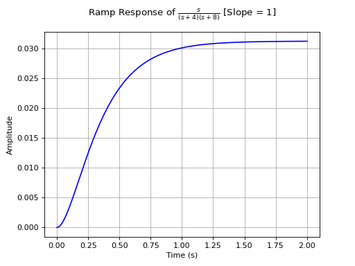
Returns the ramp response of a continuous-time system.

Ramp function is defined as the straight line passing through origin (\(f(x) = mx\)). The slope of the ramp function can be varied by the user and the default value is 1.

Parameters:

system : SISOLinearTimeInvariant type

The LTI SISO system for which the Ramp Response is to be computed.

slope : Number, optional

The slope of the input ramp function. Defaults to 1.

color : str, tuple, optional

The color of the line. Default is Blue.

show : boolean, optional

If True, the plot will be displayed otherwise the equivalent matplotlib plot object will be returned. Defaults to True.

lower_limit : Number, optional

The lower limit of the plot range. Defaults to 0.

upper_limit : Number, optional

The upper limit of the plot range. Defaults to 10.

prec : int, optional

The decimal point precision for the point coordinate values. Defaults to 8.

show_axes : boolean, optional

If True, the coordinate axes will be shown. Defaults to False.

grid : boolean, optional

If True, the plot will have a grid. Defaults to True.

Examples

>>> from sympy.abc import s
>>> from sympy.physics.control.lti import TransferFunction
>>> from sympy.physics.control.control_plots import ramp_response_plot
>>> tf1 = TransferFunction(s, (s+4)*(s+8), s)
>>> ramp_response_plot(tf1, upper_limit=2)   

(png, hires.png, pdf)

See also

step_response_plot, impulse_response_plot

References

[R733]

https://en.wikipedia.org/wiki/Ramp_function

control_plots.ramp_response_numerical_data(

slope=1,

prec=8,

lower_limit=0,

upper_limit=10,

**kwargs,

)

Returns the numerical values of the points in the ramp response plot of a SISO continuous-time system. By default, adaptive sampling is used. If the user wants to instead get an uniformly sampled response, then adaptive kwarg should be passed False and n must be passed as additional kwargs. Refer to the parameters of class sympy.plotting.series.LineOver1DRangeSeries for more details.

Parameters:

system : SISOLinearTimeInvariant

The system for which the ramp response data is to be computed.

slope : Number, optional

The slope of the input ramp function. Defaults to 1.

prec : int, optional

The decimal point precision for the point coordinate values. Defaults to 8.

lower_limit : Number, optional

The lower limit of the plot range. Defaults to 0.

upper_limit : Number, optional

The upper limit of the plot range. Defaults to 10.

kwargs :

Additional keyword arguments are passed to the underlying sympy.plotting.series.LineOver1DRangeSeries class.

Returns:

tuple : (x, y)

x = Time-axis values of the points in the ramp response plot. NumPy array. y = Amplitude-axis values of the points in the ramp response plot. NumPy array.

Raises:

NotImplementedError

When a SISO LTI system is not passed.

When time delay terms are present in the system.

ValueError

When more than one free symbol is present in the system. The only variable in the transfer function should be the variable of the Laplace transform.

When lower_limit parameter is less than 0.

When slope is negative.

Examples

>>> from sympy.abc import s
>>> from sympy.physics.control.lti import TransferFunction
>>> from sympy.physics.control.control_plots import ramp_response_numerical_data
>>> tf1 = TransferFunction(s, s**2 + 5*s + 8, s)
>>> ramp_response_numerical_data(tf1)   
(([0.0, 0.12166980856813935,..., 9.861246379582118, 10.0],
[1.4504508011325967e-09, 0.006046440489058766,..., 0.12499999999568202, 0.12499999999661349]))

See also

ramp_response_plot

Nyquist Plot

control_plots.nyquist_plot(

initial_omega=0.01,

final_omega=100,

show=True,

color='b',

**kwargs,

)

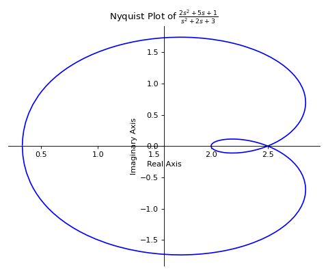
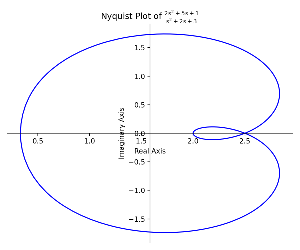
Generates the Nyquist plot for a continuous-time system.

Parameters:

system : SISOLinearTimeInvariant

The LTI SISO system for which the Nyquist plot is to be generated.

initial_omega : float, optional

The starting frequency value. Defaults to 0.01.

final_omega : float, optional

The ending frequency value. Defaults to 100.

show : bool, optional

If True, the plot is displayed. Default is True.

color : str, optional

The color of the Nyquist plot. Default is ‘b’ (blue).

grid : bool, optional

If True, grid lines are displayed. Default is False.

**kwargs

Additional keyword arguments for customization.

Examples

>>> from sympy.abc import s
>>> from sympy.physics.control.lti import TransferFunction
>>> from sympy.physics.control.control_plots import nyquist_plot
>>> tf1 = TransferFunction(2*s**2 + 5*s + 1, s**2 + 2*s + 3, s)
>>> nyquist_plot(tf1)   

(png, hires.png, pdf)

See also

nichols_plot, bode_plot

Nichols Plot

control_plots.nichols_plot(

initial_omega=0.01,

final_omega=100,

show=True,

color='b',

**kwargs,

)

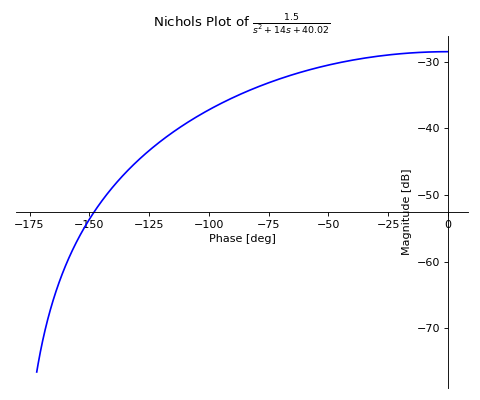
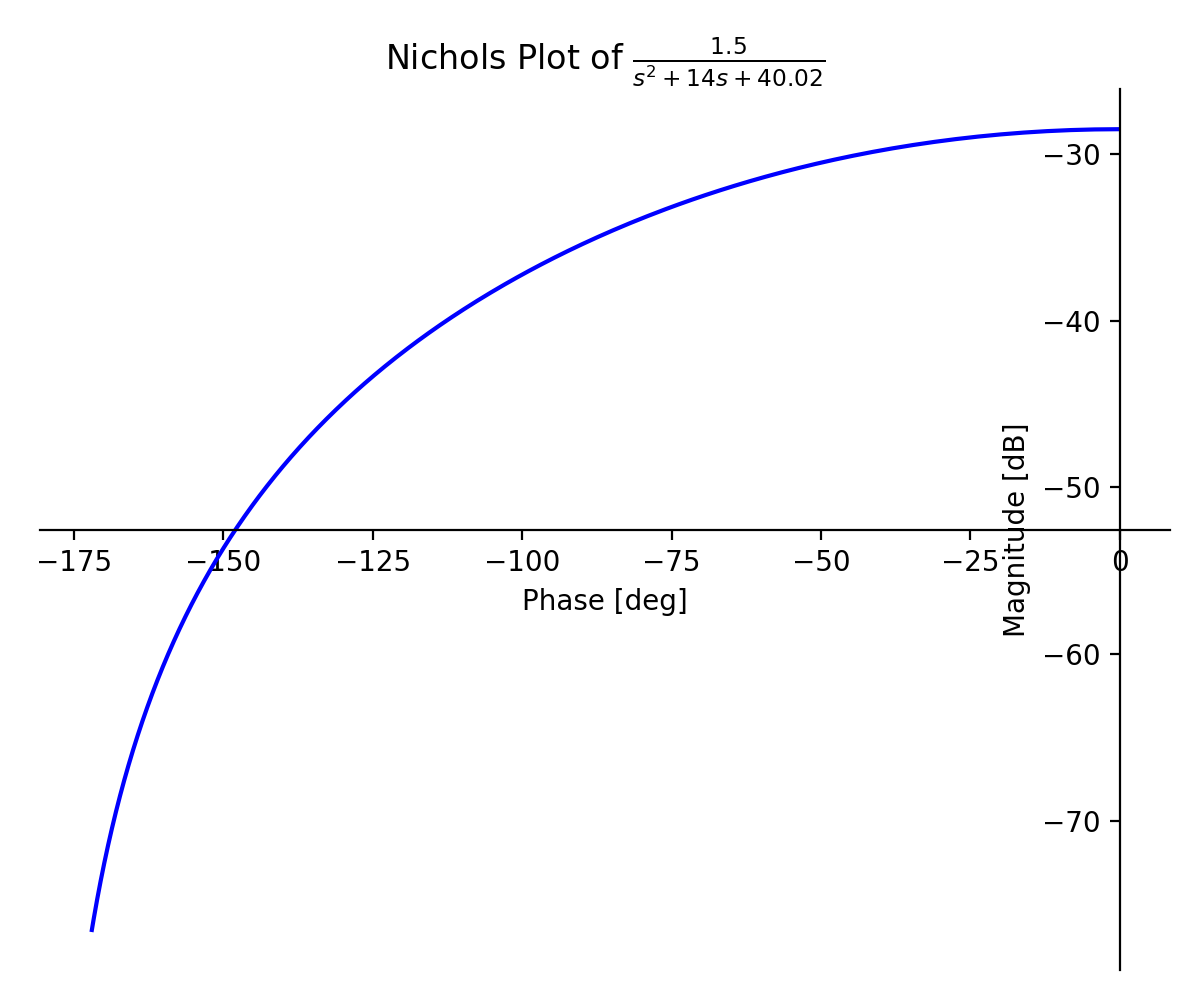
Generates the Nichols plot for a LTI system.

Parameters:

system : SISOLinearTimeInvariant

The LTI SISO system for which the Nyquist plot is to be generated.

initial_omega : float, optional

The starting frequency value. Defaults to 0.01.

final_omega : float, optional

The ending frequency value. Defaults to 100.

show : bool, optional

If True, the plot is displayed. Default is True.

color : str, optional

The color of the Nyquist plot. Default is ‘b’ (blue).

grid : bool, optional

If True, grid lines are displayed. Default is False.

**kwargs

Additional keyword arguments for customization.

Examples

>>> from sympy.abc import s
>>> from sympy.physics.control.lti import TransferFunction
>>> from sympy.physics.control.control_plots import nichols_plot
>>> tf1 = TransferFunction(1.5, s**2+14*s+40.02, s)
>>> nichols_plot(tf1)   

(png, hires.png, pdf)

See also

nyquist_plot, bode_plot