Column (Docstrings)
This module can be used to solve column displacement problems using singularity functions in mechanics.
- class sympy.physics.continuum_mechanics.column.Column(
- length,
- elastic_modulus,
- area,
- variable=x,
- base_char='C',
A column is a structural element that withstands axial loading primarily through compression. Columns are characterized by their length, material and cress-sectional area.
Note
A consistent sign convention must be used when solving these problems. Applied forces are positive when aimed in the positive x-direction. Normal forces are positive when they lead to extension, and negative when they lead to compression.
Note
The columns are set up horizontally, from left to right. This is due to it then having better compatibility with the 2-Dimensional module, where all objects are projected horizontally.
Examples
The is a column with a length of 20 meters. It has an area of 0.75 m^2 and an elastic modulus of 20.000 kN/m^2. The column is fixed at both ends. From x = 0 to x = 10 there is a constant distributed load of 5 kN/m. At x = 12 and x = 16 there are point loads of 20 kN. Loads aiming to the right are positive, and positive axial forces lead to extension.
>>> from sympy.physics.continuum_mechanics.column import Column
>>> c = Column(20, 20000, 0.75)
>>> c.apply_support(0)
>>> c.apply_support(20)
>>> c.apply_load(5, 0, 0, end=10)
>>> c.apply_load(20, 12, -1)
>>> c.apply_load(20, 16, -1)
>>> c.applied_loads
[(5, 0, 0, 10), (20, 12, -1, None), (20, 16, -1, None)]
>>> c.load
R_0*SingularityFunction(x, 0, -1) + R_20*SingularityFunction(x, 20, -1)
+ 5*SingularityFunction(x, 0, 0) - 5*SingularityFunction(x, 10, 0)
+ 20*SingularityFunction(x, 12, -1) + 20*SingularityFunction(x, 16, -1)
>>> c.solve_for_reaction_loads()
>>> c.reaction_loads
{R_0: -99/2, R_20: -81/2}
>>> c.axial_force()
99*SingularityFunction(x, 0, 0)/2 - 5*SingularityFunction(x, 0, 1)
+ 5*SingularityFunction(x, 10, 1) - 20*SingularityFunction(x, 12, 0)
- 20*SingularityFunction(x, 16, 0) + 81*SingularityFunction(x, 20, 0)/2
>>> c.extension()
0.0033*SingularityFunction(x, 0, 1) - 0.000166666666666667*SingularityFunction(x, 0, 2)
+ 0.000166666666666667*SingularityFunction(x, 10, 2) - 0.00133333333333333*SingularityFunction(x, 12, 1)
- 0.00133333333333333*SingularityFunction(x, 16, 1) + 0.0027*SingularityFunction(x, 20, 1)
- property applied_loads
Returns a list of all loads applied to the column. Each load in the list is a tuple of form (value, start, order).
Examples
There is a column of length L, area A and elastic modulus E. It is supported at both ends of the column and in the middle. There is a positive force F applied to the column at 1/4 * L and 3/4 * L.
>>> from sympy.physics.continuum_mechanics.column import Column
>>> from sympy.core.symbol import symbols
>>> L, E, A, F = symbols('L E A F')
>>> c = Column(L, E, A)
>>> c.apply_support(0)
>>> c.apply_support(L / 2)
>>> c.apply_support(L)
>>> c.apply_load(F, L / 4, -1)
>>> c.apply_load(F, 3*L / 4, -1)
>>> c.applied_loads
[(F, L/4, -1, None), (F, 3*L/4, -1, None)]
- apply_load(value, start, order, end=None)[source]
This method applies a load to the column object. Only axial loads can be applied, no moments.
- Parameters:
value: Sympifyable
The value inserted should have the units [Force/(Distance**(n+1)] where n is the order of applied load. Units for applied loads:
For point loads: kN*m
For constant distributed load: kN/m
For ramp loads: kN/m**2
For parabolic ramp loads: kN/m**3
And so on.
loc: Sympifyable
The starting point of the applied load. For point loads this is simply the location.
order: Integer
The order of the singularity function of the applied load.
For point loads, order =-1
For constant distributed load, order = 0
For ramp loads, order = 1
For parabolic ramp loads, order = 2
… so on.
Examples
There is a column of 10 meters, area A and elastic modulus E. It is supported only at the left side. There is a negative point load of 10 kN applied to the column at the right end. A positive point load of 5 kN is applied to the left end.
>>> from sympy.physics.continuum_mechanics.column import Column
>>> from sympy.core.symbol import symbols
>>> E, A = symbols('E A')
>>> c = Column(10, E, A)
>>> c.apply_support(0)
>>> c.apply_load(-10, 10, -1)
>>> c.applied_loads
[(-10, 10, -1, None)]
>>> c.apply_load(5, 0, -1)
>>> c.applied_loads
[(-10, 10, -1, None), (5, 0, -1, None)]
- apply_support(loc)[source]
Add supports to the system.
Supports can be defined in two ways in the module:
1. Using
apply_support()Automatically applies all required boundary conditions internally and generates aSymbol(R_loc)representing the reaction load at the specified support location.2. Manual method Add a reaction symbol as a load using
apply_load()and manually specify the corresponding boundary conditions.This applies a support that is fixed in the horizontal direction. using the apply_support() method
- Parameters:
loc: Sympifyable
Location at which the fixed support is applied.
Examples
There is a column of 10 meters. It has an area A and elastic modulus E. The column has fixed supports at both ends.
>>> from sympy.physics.continuum_mechanics.column import Column
>>> from sympy.core.symbol import symbols
>>> E, A = symbols('E A ')
>>> c = Column(10, E, A)
>>> c.apply_support(0)
>>> c.apply_support(10)
>>> c.apply_load(-10, 10, -1)
>>> print(c.load)
R_0*SingularityFunction(x, 0, -1) + R_10*SingularityFunction(x, 10, -1)
    - 10*SingularityFunction(x, 10, -1)
This applies a support that is fixed in the horizontal direction. using the apply_load() method
>>> from sympy.physics.continuum_mechanics.column import Column
>>> from sympy.core.symbol import symbols
>>> E, A = symbols('E A ')
>>> R_0, R_10 = symbols('R_0 R_10')
>>> c = Column(10, E, A)
>>> c.apply_load(R_0,0,-1)   # Reaction applied as a point load
>>> c.apply_load(R_10,10,-1) # Reaction applied as a poinnt load
>>> c._bc_extension.append(0) # boundary conditions are added manually
>>> c._bc_extension.append(10) # boundary conditions are added manually
>>> c.apply_load(-10, 10, -1)
>>> print(c.load)
R_0*SingularityFunction(x, 0, -1) + R_10*SingularityFunction(x, 10, -1)
    - 10*SingularityFunction(x, 10, -1)
- apply_telescope_hinge(loc)[source]
Applies a telescope hinge at the given location. At this location, the column is free to move in the axial direction.
- Parameters:
loc: Sympifyable
Location at which the telescope hinge is applied.
Examples
There is a column with a length of 10 meters, elastic modulus E and area A. At x = 5 the column is loaded axially by a point load of 10 kN. At x = 8, there is a telescope hinge.
>>> from sympy.physics.continuum_mechanics.column import Column
>>> c = Column(10, 20000, 0.5)
>>> c.apply_support(0)
>>> c.apply_support(10)
>>> c.apply_telescope_hinge(8)
>>> c.apply_load(10, 5, -1)
>>> c.solve_for_reaction_loads()
>>> c.reaction_loads
{R_0: -10, R_10: 0}
>>> c.hinge_extensions
{u_8: 1/200}
- property area
Returns the cross-sectional area of the column.
- axial_force()[source]
Returns a singularity function expression that represents the axial forces in the column.
Examples
A column with a length of 10 meters, elastic modulus E and area A is supported at both ends and in the middle. At x = 3 the column is loaded by a point load of magnitude -1 kN. Between x = 5 and x = 10 the column is loaded by a uniform distributed load of -1 kN/m.
>>> from sympy.physics.continuum_mechanics.column import Column
>>> from sympy.core.symbol import symbols
>>> E, A = symbols('E A')
>>> c = Column(10, E, A)
>>> c.apply_support(0)
>>> c.apply_support(5)
>>> c.apply_support(10)
>>> c.apply_load(-5, 3, -1)
>>> c.apply_load(-1, 5, 0, end=10)
>>> c.axial_force()
C_N - R_0*SingularityFunction(x, 0, 0) - R_10*SingularityFunction(x, 10, 0)
    - R_5*SingularityFunction(x, 5, 0) + 5*SingularityFunction(x, 3, 0)
    + SingularityFunction(x, 5, 1) - SingularityFunction(x, 10, 1)
>>> c.solve_for_reaction_loads()
>>> c.axial_force()
-2*SingularityFunction(x, 0, 0) + 5*SingularityFunction(x, 3, 0)
    - 11*SingularityFunction(x, 5, 0)/2 + SingularityFunction(x, 5, 1)
    - 5*SingularityFunction(x, 10, 0)/2 - SingularityFunction(x, 10, 1)
- property elastic_modulus
Returns the elastic modulus of the column
- extension()[source]
Returns a singularity function expression that represents the extension of the column.
Examples
A column with a length of 10 meters has an elastic modulus of 210000 kN/m^2 and an area of 1 m^2. It is supported at both ends and is loaded by a point load of 10 kN at x = 5.
>>> from sympy.physics.continuum_mechanics.column import Column
>>> c = Column(10, 210000, 1)
>>> c.apply_support(0)
>>> c.apply_support(10)
>>> c.apply_load(10, 5, -1)
>>> c.extension()
C_N*x + C_u - R_0*SingularityFunction(x, 0, 1)/210000
- R_10*SingularityFunction(x, 10, 1)/210000 - SingularityFunction(x, 5, 1)/21000
>>> c.solve_for_reaction_loads()
>>> c.extension()
SingularityFunction(x, 0, 1)/42000 - SingularityFunction(x, 5, 1)/21000
+ SingularityFunction(x, 10, 1)/42000
- property hinge_extensions
Returns the hinge extensions as dictionary.
- property length
Returns the length of the column.
- property load
Returns the load equation qx of the applied loads and reaction forces using singularity functions.
Examples
There is a column of length L, area A and elastic modulus E. It is supported at both ends of the column and in the middle. There is a positive force F applied to the column at 1/4 * L and 3/5 * L.
>>> from sympy.physics.continuum_mechanics.column import Column
>>> from sympy.core.symbol import symbols
>>> L, E, A, F = symbols('L E A F')
>>> c = Column(L, E, A)
>>> c.apply_support(0)
>>> c.apply_support(L / 2)
>>> c.apply_support(L)
>>> c.apply_load(F, L / 4, -1)
>>> c.apply_load(F, 3*L / 4, -1)
>>> c.load
F*SingularityFunction(x, L/4, -1) + F*SingularityFunction(x, 3*L/4, -1)
    + R_0*SingularityFunction(x, 0, -1) + R_L*SingularityFunction(x, L, -1)
    + R_L/2*SingularityFunction(x, L/2, -1)
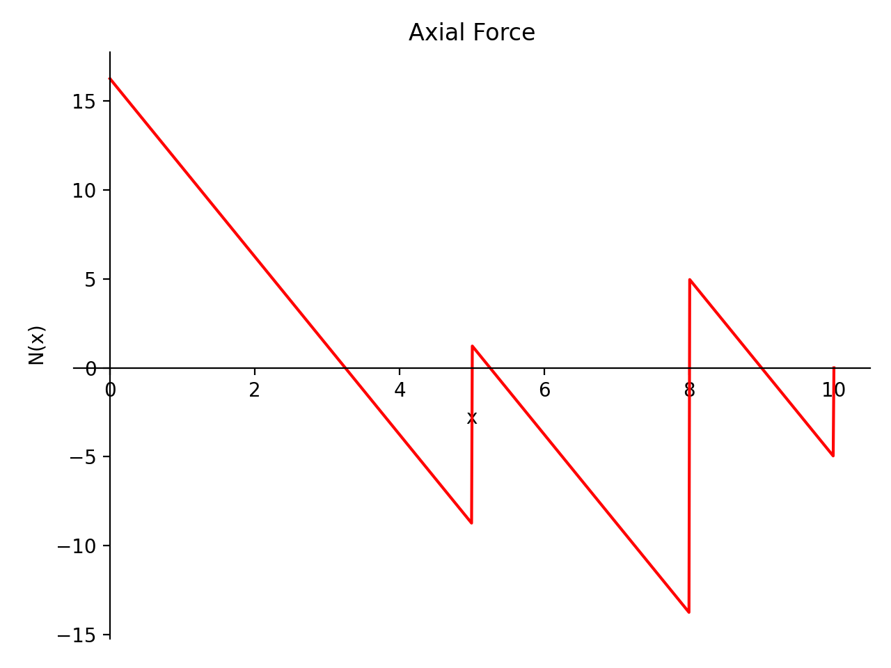
- plot_axial_force()[source]
Returns a plot for the axial forces in the column.
Examples
There is a column with a length of 10 meters, an elastic modulus of 210000 kN/m^2 and an area of 1 m^2. It is supported at x = 0, x = 8 and x = 10. There is a uniform distributed load of 5 kN applied to the whole column. Furthermore, there are point loads of -10 kN and 5 kN at x = 5 and x = 8, respectively.
Negative axial force loads to compression, and positive axial force leads to extension.
>>> from sympy.physics.continuum_mechanics.column import Column
>>> c = Column(10, 210000, 1)
>>> c.apply_support(0)
>>> c.apply_support(8)
>>> c.apply_support(10)
>>> c.apply_load(5, 0, 0, end=10)
>>> c.apply_load(-10, 5, -1)
>>> c.apply_load(5, 8, -1)
>>> c.solve_for_reaction_loads()
>>> c.plot_axial_force()
Plot object containing:
[0]: cartesian line: 65*SingularityFunction(x, 0, 0)/4
- 5*SingularityFunction(x, 0, 1) + 10*SingularityFunction(x, 5, 0)
+ 75*SingularityFunction(x, 8, 0)/4 + 5*SingularityFunction(x, 10, 0)
+ 5*SingularityFunction(x, 10, 1) for x over (0.0, 10.0)

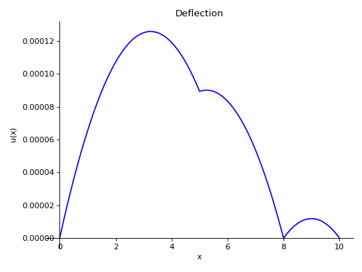
- plot_extension()[source]
Returns a plot for the extensions in the column. To plot the extension, numeric values for elastic modulus E and are A should be provided.
Examples
There is a column with a length of 10 meters, an elastic modulus of 210000 kN/m^2 and an area of 1 m^2. It is supported at x = 0, x = 8 and x = 10. There is a uniform distributed load of 5 kN applied to the whole column. Furthermore, there are point loads of -10 kN and 5 kN at x = 5 and x = 8, respectively.
>>> from sympy.physics.continuum_mechanics.column import Column
>>> c = Column(10, 210000, 1)
>>> c.apply_support(0)
>>> c.apply_support(8)
>>> c.apply_support(10)
>>> c.apply_load(5, 0, 0, end=10)
>>> c.apply_load(-10, 5, -1)
>>> c.apply_load(5, 8, -1)
>>> c.solve_for_reaction_loads()
>>> c.plot_extension()
Plot object containing:
[0]: cartesian line: 13*SingularityFunction(x, 0, 1)/168000
- SingularityFunction(x, 0, 2)/84000 + SingularityFunction(x, 5, 1)/21000
+ SingularityFunction(x, 8, 1)/11200 + SingularityFunction(x, 10, 1)/42000
+ SingularityFunction(x, 10, 2)/84000 for x over (0.0, 10.0)

- property reaction_loads
Returns the reactions loads as dictionary.
- remove_load(value, start, order, end=None)[source]
Removes an applied load.
Examples
There is a column with a length of 4 meters, area A and elastic modulus E. A point load of -2 kN is applied at x = 2 and a constant distributed load of 2 kN/m is applied along the whole column. Later, the point load is removed.
>>> from sympy.physics.continuum_mechanics.column import Column
>>> from sympy.core.symbol import symbols
>>> E, A = symbols('E A')
>>> c = Column(4, E, A)
>>> c.apply_load(-2, 2, -1)
>>> c.apply_load(2, 0, 0, end=4)
>>> print(c.load)
2*SingularityFunction(x, 0, 0) - 2*SingularityFunction(x, 2, -1) - 2*SingularityFunction(x, 4, 0)
>>> c.remove_load(-2, 2, -1)
>>> print(c.load)
2*SingularityFunction(x, 0, 0) - 2*SingularityFunction(x, 4, 0)
- solve_for_reaction_loads(*reactions)[source]
This method solves the horizontal reaction loads and unknown displacement jumps due to telescope hinges.
- Parameters:
reactions: If supports of the system are applied manually using apply_load()
method The reaction load symbols to be passed as reactions.
Examples
A column of 10 meters long, with area A and elastic modulus E is supported at both ends. A distributed load of -5 kN/m is applied to the whole column. A point load of -10 kN is applied at x = 4.
>>> from sympy.physics.continuum_mechanics.column import Column
>>> from sympy.core.symbol import symbols
>>> E, A = symbols('E A')
>>> c = Column(10, A, E)
>>> c.apply_support(0)
>>> c.apply_support(10)
>>> c.apply_load(-5, 0, 0, end=10)
>>> c.apply_load(-10, 4, -1)
>>> c.solve_for_reaction_loads()
>>> c.reaction_loads
{R_0: 31, R_10: 29}
The same example when applied applied supports using manual method apply_load()
>>> from sympy.physics.continuum_mechanics.column import Column
>>> from sympy.core.symbol import symbols
>>> E, A = symbols('E A')
>>> R, G = symbols('R G')
>>> c = Column(10, A, E)
>>> c.apply_load(R,0,-1) # applied reaction load as a point load
>>> c.apply_load(G,10,-1) # applied reaction load as a point load
>>> c._bc_extension.append(0) # boundary conditions are added manually
>>> c._bc_extension.append(10) # boundary conditions are added manually
>>> c.apply_load(-5, 0, 0, end=10)
>>> c.apply_load(-10, 4, -1)
>>> c.solve_for_reaction_loads(R,G) # Reaction loads need to be passed.
>>> c.reaction_loads
{G: 29, R: 31}